Draft 2: Added some features.
Over the past year this blog has argued for a materialist political economy. The argument has three layers, and each one rests on the one before it.
- Physical. Labor value is conserved when goods are exchanged. That one fact is supposed to make prices follow values and split the population into two classes by how much money they hold.
- Social. Class relations drive capitalism’s dynamics. The profit rate tends to fall, a reserve army of the unemployed holds wages down, and people turn to radical politics when their living standards fall.
- Programmatic. Democratic planning would remove those dynamics. Its tools are a job guarantee, labor vouchers that cannot circulate like money, a government divided against itself, and a cap on private assets.
In this post I put those claims to the test. They come from seven earlier posts:
- Materialist economics, part 1: mechanical materialism
- Materialist economics, part 3: accountable planning
- Materialist economics, part 4: objections and responses
- Philosophies of contradiction: Marx contra Buddha
- Structural dialectics
- Contemporary fascism is an outgrowth of capitalism
- Why leftists must focus on job creation
I have boiled those posts down to seventeen claims, or propositions: thirteen in §2 and four about finance in §9. I then wrote each mechanism behind them as a set of rules in Palimpsest, a small programming language in which a program is a list of rewrite rules (§3 explains what that means). Running the rules is running the economy. Each proposition then gets three questions:
- Does the model actually produce the claim?
- Where does its behavior change? At what limits, thresholds and tipping points does a claim stop being true?
- Do published data show the same pattern, and at a size the model can match?
Here is what I found, in brief.
Value and profit. Three things follow directly from the rules: value is conserved, the planning computation converges quickly, and wages and profits move in opposite directions. Prices do follow values, as the data show. But the model’s prices stray from values by only 0.8–3.1%, while measured deviations are 7–20%. The profit rate falls only if something fixes the wage (Okishio’s theorem holds in 18 of 18 cases I tested) or if population growth slows. Its long-run level also hits a floor once the population shrinks fast enough, and the model tells you how fast that is.
Money. Conservation alone gives the lower class an exponential distribution of money, with a Gini coefficient of 0.524. US tax data give about 0.5. Without an asset cap, though, capital income piles up far beyond the real top-1% wealth share of 32.5%. In the simulation one owner ends up with 98% of all the money.
The labor market. The bargained wage responds to unemployment with an elasticity of −0.1 at 5.5% unemployment, which is the figure economists measure. When unemployment is below 1/12 (8.3%), moving capital abroad becomes the employers’ best move. A job guarantee raises private wages by 5% at 12.5% unemployment, close to what India’s NREGA scheme did, and has no effect below 1/11 (9.1%).
Politics. Voters pick a radical gamble only after a deep loss. How deep is set by the shape of their attitude to losses (its curvature), and hardly at all by loss aversion. That fits the finding that far-right votes rise after financial crises but not after ordinary recessions. A government divided into at least 1/P independent offices cannot sustain a conspiracy, where P is the chance of an audit and a whistle-blower’s reward equals the bribe.
The whole economy. With all the mechanisms running together under capitalism, labor’s share of income falls 19.9% over 60 periods. The US share fell 20.2% from 1960 to 2026. But the model’s unemployment rises without limit, because machines replace workers faster than new investment creates jobs. An economic shock turns into a lasting radical government once right-wing “aspiration messaging” passes a sharp threshold between 0.26 and 0.27. Under planning, every route into the radical vote disappears.
Finance. When buyers can borrow a share LTV of a house’s price, a fixed stock of houses sells for S/(1 − LTV), where S is what buyers have saved. The new money goes to the people who already own the houses, and no extra output is produced. When capital gains are set against the things that break fortunes up (inheritance, bankruptcy, taxes), the rich form a Pareto class whose shape is fixed by one number, the exponent log₂(q/p). Read this way, the US top-1% wealth share implies an exponent of 1.46 in 1989, close to direct estimates of 1.48–1.55, and 1.32 in 2026. Forced selling feeds on itself only when one sale pushes the price down further than the gap between one firm’s debt and the next. In a fourth, financialized version of the economy, credit keeps people employed until a falling profit rate and interest payments bring on a crash, the kind Hyman Minsky described. In the baseline run each of these crashes produces a radical government, through the moment when credit dries up for indebted households. None does when households carry no debt. This economy elects radical governments in all 27 stress settings I tried; plain capitalism does so in 15. Inflation delays the debt crisis and deflation brings it closer. Letting firms decide when to mechanize stops unemployment rising, but it also shows that the match with the falling labor share depended on that rise.
A separate Python program recomputes every table in this post and checks it character for character (80 checks). You can also run every program in your browser, in the Palimpsest playground.
1 Introduction
My earlier posts covered mechanical materialism, accountable planning, objections and responses, philosophies of contradiction, structural dialectics, fascism as an outgrowth of capitalism, and job creation. Read together, they make one argument that runs from physics to politics.
It starts with conservation. Following Paul Cockshott, value is abstract labor time, and exchange conserves it, the way collisions conserve energy in a gas. Just as energy conservation produces regular statistical patterns in a gas, conservation of value is meant to produce regular patterns in an economy: prices close to labor values, an exponential distribution of money, and a population split into two income classes.
Class relations come next. Who owns the means of production, and who can afford to walk away from a bargain, decide how the economy moves: a falling profit rate, a reserve army of unemployed people that keeps wages down, newly created money that favors people who already own assets, and radical politics when living standards fall.
Last comes a design. Accountable planning is meant to remove those dynamics.
Every link in that chain is a claim about how something works, so every link can be stated precisely and checked. For each one I ask three things. If I state the mechanism precisely, does it produce what the posts say? Where does its behavior change? And how well do the results match the data?
Why rewrite rules? The mechanical-materialism post defines a scientific law as “regularities governing how systems change states under specified conditions”. A rewrite rule says exactly that: when you see something of this shape, replace it with something of that shape, provided these conditions hold. So I wrote the economy as rewrite rules in Palimpsest, a language built around them. Three ideas carry the whole method:
- One period of the economy is one complete rewriting of a term that holds the state of the economy.
- A feedback loop is a chain of rules through which something computed in period t comes back in period t + 1.
- To check that a cause-and-effect arrow in the diagram is real, I nudge one variable, hold every other one fixed, run the rules again and see which way the result moves.
Class analysis feeds the games. Some of the mechanisms are games, in the sense of game theory. Class position decides who the players are, what each can fall back on if bargaining breaks down, and how much is at stake. Under capitalism a worker’s fallback is the reserve army: if she loses this job, will she find another? A job guarantee replaces that fallback with a public job. That one change alters the wage bargain and the game between labor and capital, and through prospect theory, a model of how people weigh gains and losses, it changes how many voters back a radical gamble.
1.1 Summary of findings
The bookkeeping and the equilibria hold up. Conservation, the exponential law, the transfer to whoever gets new money first (the Cantillon effect), the fact that vouchers cannot circulate, and the job guarantee’s effect on employers all follow directly from the rules.
Claims stated without conditions turn out to have conditions. The falling profit rate, the radical coalition, the job guarantee’s power and the patronage spiral each hold only for some values of the model’s settings. The model shows where the boundary lies.
The patterns match the data, but some of the sizes do not. Without fitting anything to the data, the model comes close on the wage curve, the decline of labor’s share, the Gini coefficient of the lower class and the job guarantee’s effect on wages. It misses on how far prices stray from values, on how concentrated wealth is, and on the trend in unemployment. In each miss the model points in the right direction, and something is missing from it.
Finance makes the political results clearer. A financial crisis becomes a radical government at the moment credit dries up for indebted households, because borrowing had lifted the living standard people measure themselves against, and the crunch takes it away. Inflation delays the second debt crisis but cannot prevent the first. Capital gains produce a Pareto class, and policy sets its size. Adding two missing mechanisms, the breaking-up of fortunes and mechanization that responds to wages, repairs two of the misses above. The second repair also shows that the labor-share match depended on unemployment rising (§9).
1.2 How this post is organized
Section 2 lists the claims as propositions T1–T13 and explains the three tests; §9 adds T14–T17. Section 3 introduces Palimpsest. Sections 4–8 follow the posts from physics to politics: value, prices and profit (§4), money (§5), the labor market (§6), politics (§7), and the whole economy with every mechanism running at once, in three versions (§8). Section 9 adds finance: credit money, capital gains, debt deflation and a fourth, financialized version of the economy (T14–T17), along with two more mechanisms the first version left out, mechanization that responds to wages and the mobility of capital. Section 10 collects the verdicts, §11 explains how to reproduce everything, §12 lists the limitations, and §13 sums up.
2 The claims and how I test them
2.1 Seventeen propositions
The posts draw on three books in particular:
- Classical Econophysics (Cockshott, Cottrell, Michaelson, Wright and Yakovenko, 2009), which treats value, money and profit with the tools of statistical physics.
- How the World Works (Cockshott, 2019), a history of human labor that includes a demographic theory of the profit rate.
- The Logic of Political Survival (Bueno de Mesquita, Smith, Siverson and Morrow, 2003). Its “selectorate theory” explains how leaders stay in power by rewarding the group whose support they need. I use it for the claims about party-states, patronage and divided government.
I reduced the posts to thirteen propositions, and §9 adds four about finance. The table quotes the post each one comes from.
| proposition | post (quoted) | tested in | |
|---|---|---|---|
| T1 | Value is conserved in exchange; surplus value cannot arise from exchange | mechanical materialism: “in the exchange of commodities, abstract socially necessary labor time is conserved” | §4.1 |
| T2 | Labor values predict market prices | mechanical materialism: “labor values reliably predict prices” | §4.2 |
| T3 | Conservation yields an exponential distribution of money, and capital income a Pareto upper class | mechanical materialism: “the lower approximately 97% … follows an exponential law … the upper approximately 3% follows a Pareto power law” | §5.1–5.2 |
| T4 | Money creation redistributes real claims toward asset holders | mechanical materialism: it “does not create new value but redistributes existing claims on real output” | §5.3 |
| T5 | The rate of profit tends to fall | mechanical materialism: “the rate of profit tends to fall over the long run” | §4.3, §8.3 |
| T6 | Planning is a fast contractive computation | accountable planning: “By approximately the twentieth pass they converge” | §4.1 |
| T7 | Quadratic voting replaces the purchasing-power filter and protects intense minorities | accountable planning: it “directly replaces the purchasing-power filter with a democratic one” | §7.5 |
| T8 | A job guarantee breaks employers’ power | accountable planning: capitalists “must offer conditions attractive enough to compete with the government sector” | §6.1–6.3 |
| T9 | A divided government cannot conspire | accountable planning: it “is divided within itself … so that it cannot conspire against the people” | §7.3–7.4 |
| T10 | Vouchers and an asset cap prevent accumulation | accountable planning: vouchers “cannot be lent, invested, or accumulated” | §5.2–5.3 |
| T11 | Falling living standards and inflation drive voters to radical, authoritarian options | fascism: “The more radical side will always form the more powerful coalition”; accountable planning on inflation as an existential threat | §7.1, §8.2, §8.4 |
| T12 | Right-wing patronage employment produces a self-reinforcing spiral | job creation: “The right buys off every community leader … It’s a downward spiral” | §7.2, §8.4–8.5 |
| T13 | Planning defuses authoritarian politics | accountable planning: “Because workers’ purchasing power rises rather than erodes, the existential anxiety that drives populations toward authoritarian leaders is defused” | §8.2, §8.4–8.6 |
| T14 | Credit creates money and inflates asset prices, not output | mechanical materialism: “New money bids up the price of housing and equities without a corresponding increase in the real output of the economy” | §9.1 |
| T15 | Compounding capital gains produce the Pareto class, which reform cannot remove | mechanical materialism: “The Pareto (superthermal) class corresponds to compounding capital-gains income” | §9.2 |
| T16 | Nominal debt makes deflation a self-reinforcing spiral, so the system needs inflation, which cuts real pay | accountable planning: “The system requires that the purchasing power of money be deliberately eroded as a condition of its own stability” | §9.3–9.4 |
| T17 | Debt deepens economic desperation and the turn to authoritarian options | accountable planning: insecurity is “an existential threat in the same register as mortality”; this evaluation’s first version: “Increasing debt increases desperation” | §9.5 |
Two posts supply method rather than claims.
- Philosophies of contradiction follows the Italian philosopher Lucio Colletti in treating class conflict as a real opposition between forces, rather than a logical contradiction, and it describes how an alternative can be “foreclosed”, shut off before it can happen. The real opposition shows up in the model as the trade-off between wages and profits (§4.2). Foreclosure shows up as a window for change that closes once a radical government takes office (§8.6).
- Structural dialectics defines tests for when one social form should give way to another: viability, necessity, Phase Inversion, warrant and synthesis. I apply them to the full model (§8.6).
The objections post adds a rule for counting an hour of skilled labor as several hours of simple labor (§4.1).
2.2 Three tests
Every result in this post comes from an assertion or a printed table in one of the programs listed in Appendix B. An assertion is a line the program checks; if it is false, the program stops with an error.
Test 1: does the model produce the claim? I use four verdicts.
- Derived: the proposition follows from the rules for every setting of the parameters.
- Reproduced: it holds at the model’s chosen settings.
- Qualified: it holds only under an extra condition, which the model makes visible.
- Contradicted: it fails.
Test 2: where does the behavior change? I look for limits, thresholds and tipping points, and pin them down precisely.
Test 3: what do the data say? Do published measurements show the pattern the model produces, at a size the model can match?
I did not fit the model to any data. Its settings come from its own steady-state algebra (§8.1) or from the posts, so when it matches the data, that is a test of the mechanism rather than of my choice of numbers. Each empirical figure used in a comparison is stored, with its source, in examples/me-evidence.pal.
3 Method: feedback loops as rewrite rules in Palimpsest
Palimpsest is a term-rewriting language with an interpreter written in Rust. A program has four parts:
- a set of rewrite rules;
- strategies, which say where and in what order to apply the rules;
- a starting term, called
main; - a list of commands.
A program may also rewrite its own source file, but only if it declares that it is allowed to. Palimpsest runs in the browser too, in the Palimpsest playground. There, a Python port of the interpreter runs under Pyodide (Python compiled to WebAssembly), and it gives the same output and the same step counts as the Rust interpreter on every example program.
3.1 Terms, rules and strategies
A term is a symbol, a string, a number or a list in parentheses. A rule has a name, a pattern on the left, a replacement on the right and, optionally, conditions after where:
rule NAME : LHS => RHS where CLAUSE, CLAUSE, ...
Pattern variables come in three kinds:
?xmatches any single piece of a term.?xs...matches several list items in a row.!xis strict: the matching piece is simplified completely (put in “normal form”) before the pattern is tried.
A condition is either a test, which must come out true, or a binding ?v <- EXPR, which computes a value and names it. Conditions are worked out from left to right, and they can use every rule in the program.
The model uses one strategy throughout. It always rewrites the outermost, leftmost piece it can, which computer scientists call normal-order reduction:
strategy eval = outermost(prim + rules)
Each rewriting step uses up one unit of “fuel”, and a program declares its budget with #fuel N. Running out of fuel is an error, never a silent stop. The fuel left at the end works as a fingerprint of the whole computation: if two runs leave different amounts, they did different things.
3.2 Numbers, records and commands
Numbers are exact. An integer can be any size, and a fraction is written n/d. A number whose value is a whole number is always stored as one, so 6/3 simply is 2, and two numbers are equal exactly when their values are. The built-in operations include exact division q/, num and den (numerator and denominator), expt (powers), isqrt (integer square root) and round-to x K, which rounds x to the nearest multiple of 1/K. Nothing is rounded unless the program asks for it.
Records hold the economy’s state, as in (rec (K 270) (kap 3) …). You read a field with @ and change one with set@, put@ or add@.
Commands. A program file starts with settings such as #fuel and #memo, followed by commands:
show TERM with S // print the normal formdisplay TERM with S // print a string normal form as textassert TERM with S // PASS iff the normal form is true; a FAIL exits non-zerolet $NAME = TERM with S // normalize once, substitute $NAME in later commandsrewrite self with S // rewrite main and write the program back to its file
rewrite self writes the file in one step, keeps a copy of the old version so the change can be undone, and writes nothing when run with --dry-run. A program that moves its economy forward one step at a time stops changing once its condition fails. Rewriting it again then leaves the file byte for byte the same, so the program has become a quine, a program whose output is its own source.
#memo makes the interpreter remember pieces it has already simplified, which saves work: 400 periods of the small example below take 10,568 steps instead of 29,505. --trace N prints the first N rewriting steps, and --stats reports which rules did the work.
3.3 A worked example: one feedback loop, step by step
examples/me-tour.pal is the smallest complete example of the method. It is one loop: capital K decides employment E, employment decides unemployment u, unemployment decides the wage w, the wage decides profit, and profit becomes next period’s capital.
- Capital K employs E = min(100, K/3) of N = 100 workers.
- Unemployment u = 1 − E/N sets the bargained wage share w(u) (§6.1).
- Three-fifths of profit, (1 − w)E, is invested, and capital wears out at 3% a period.
rule wage : (wage !u) => (q/ (+ 1/5 (* 4/5 (* ?u 2/5))) (+ 1/5 (* ?u 4/5)))rule step : (step (st ?t ?k)) => (st ?t1 (round-to ?k2 1000)) where ?t1 <- (+ ?t 1), ?e <- (min 100 (q/ ?k 3)), ?u <- (- 1 (q/ ?e 100)), ?w <- (wage ?u), ?k2 <- (+ (* 97/100 ?k) (* 3/5 (* (- 1 ?w) ?e)))rule run-0 : (run !s !n) => ?s where (<= ?n 0)rule run-n : (run !s !n) => (run (step ?s) (- ?n 1)) where (> ?n 0)
Running palimpsest examples/me-tour.pal --trace 22 shows the first period (an excerpt):
      2   min: (min 100 (q/ 270 3))  =>  (if (<= 100 (q/ 270 3)) 100 (q/ 270 3))
      3   <prim>: (q/ 270 3)  =>  90
      4   <prim>: (<= 100 90)  =>  false
      5   if-false: (if false 100 (q/ 270 3))  =>  (q/ 270 3)
      6   <prim>: (q/ 270 3)  =>  90
      9   wage: (wage 1/10)  =>  (q/ (+ 1/5 (* 4/5 (* 1/10 2/5))) (+ 1/5 (* 1/10 4/5)))
     15   <prim>: (q/ 29/125 7/25)  =>  29/35
     21 step: (step (st 0 270))  =>  (st 1 (round-to 18981/70 1000))
     22 <prim>: (round-to 18981/70 1000)  =>  271157/1000
At u = 1/10 the wage share comes out as the exact fraction 29/35. The trace also shows a cost of putting off work: min copies an argument it has not evaluated yet, so the same division is done twice (steps 3 and 6). Laziness can cost much more than that. If the loop counter is not forced, it grows into (- (- … 1) 1) and every test has to work it out again, so a loop that should take linear time takes quadratic time. The strict variables !s !n prevent this, which is why every entry point in the libraries is strict.
The loop settles where investment just replaces the capital that wears out: w = 17/20, u = 1/12 and K* = 275.
4 Value, prices and profit (T1, T2, T5, T6)
This section starts with what is conserved, then asks how prices relate to it, and ends with what happens to profitability over time. The results are checked by me-value.pal (17 assertions) and me-classical.pal (8), and the thresholds come from me-extremes.pal (§X3, §X5, §X10).
The reference economy, which I call E3, has three sectors: means of production (machines and materials), necessities (what wages buy) and luxuries. A is the table of inputs each sector needs per unit of output, l is the labor each needs, and b is the workers’ consumption bundle:

4.1 Value, exchange and the plan (T1, T6)
Values and the plan. The labor value of a good is the total labor, direct and indirect, that goes into making it. Solving the input table exactly gives labor values λ = (50/31, 90/31, 36/31). A planner can find the gross output x needed for a final demand d by repeating the step x ← Ax + d until it settles. On a reconstruction of the four-sector plan in the planning post, the estimates agree to within one ton after 18 passes; the post says “approximately the twentieth pass”. For every final demand d, the value of the net product equals the living labor performed: λ·d = l·x.
Exchange. Suppose an exchange table says how much of one good trades for another. If the table is consistent (reflexive, symmetric and transitive), it has the form Tᵢⱼ = vᵢ/vⱼ for some set of values v, and any round of trades brings you back to what you started with. Break transitivity by 10% and a three-trade cycle returns 11/10 of what went in: money makes more money from trade alone, Marx’s M–C–M′, with no production involved. When exchange conserves value, trade cannot create surplus value.
Real data and skilled labor. Classical Econophysics Table 10.1 is a four-industry input–output table. From it, the labor values per dollar of output all fall within 5.65% of their average, and the value of final output equals the wage bill, 244. The objections post counts a skilled hour as 3/2 simple hours. If the people who train the skilled workers are themselves skilled, the coefficient has to be worked out as the settling point of a repeated calculation, and it comes to 7/4.
Verdict: T1 and T6 are derived. Conservation holds for every consistent exchange table and fails for every inconsistent one. How fast the plan converges depends on the largest eigenvalue (the spectral radius) of A.
4.2 Prices and the wage–profit trade-off (T2)
The profit rate, pinned down exactly. When every sector earns the same profit rate r*, prices p satisfy p = (1 + r)p(A + b⊗l). I never compute an eigenvalue. Instead I halve an interval of possible values of r again and again, and at each step I decide exactly, using the Hawkins–Simon test on fractions, which half contains r*. After 30 halvings, r* ∈ [0.22849294, 0.22849294).
Two theorems hold on every wage bundle I tried:
- The Fundamental Marxian Theorem (Morishima, 1973) says profits are positive if and only if workers are exploited, in the sense that they produce more value than they consume. It holds on 21 wage bundles and on all 64 bundles of a grid, including the edge case λ·b = 1, where r* = 0.
- The Generalized Commodity Exploitation Theorem says the same is true of every basic good, not just labor: on the same bundles, each basic commodity is “exploited” exactly when r* > 0. So the theorems do not single labor out. The case for labor as the source of value has to rest on evidence.
The real opposition. Measure the wage in units of the net product, and it falls from 1 at r = 0 to 0.0174 at r = 1.9 (Figure 1). Whatever one class gains, the other loses. Along the same curve, the average gap between prices and values, measured as the mean absolute weighted deviation (MAWD), rises from 0 at r = 0 to 0.0349 at r = 1. If every sector uses capital and labor in the same proportions, the gap is zero at every r.
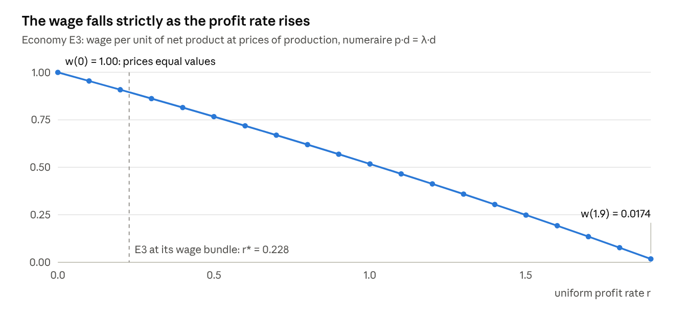
me-value.pal §3.5. Exact rationals shown to four decimals).What the data say. The evidence supports T2 on direction and partly on size.
- Cockshott and Cottrell (1997) report a correlation of 0.977 between prices and labor values for the UK. Zachariah (2006) reports 0.942–0.986 for the seven OECD economies listed in Classical Econophysics.
- Shaikh (1998) measures a MAWD of 9.2% for the US, and Classical Econophysics reports 7.1–10.5% for 1947–1972. Işıkara and Mokre (2022), using 42 countries, find deviations that are small and stable; the mechanical-materialism post quotes them at 10–20%.
The model’s deviations are too small: 0.8% in E3 and 3.1% for Table 10.1, three to eleven times below Shaikh’s figure. The reason is aggregation. Three or four sectors cannot capture how much the mix of capital and labor varies across the 40 to 100 industries in real tables.
Verdict: T2 is derived in structure and supported by the data, but the model’s deviations are too small.
4.3 The falling rate of profit (T5)
One of Marx’s best-known claims is that the profit rate tends to fall over time. The model can look at this in three ways, over three time spans.
New techniques: Okishio’s theorem. I tested eighteen changes that replace labor with machinery. Capitalists adopt a change if and only if it lowers their cost per unit at current prices.
- If the real wage stays fixed, Okishio’s theorem holds in all 18: every change capitalists adopt raises the profit rate.
- If instead the rate of exploitation stays fixed, the profit rate falls after 11 of the 14 changes they adopt.
So whether the profit rate falls depends on what happens to wages. The tendency is only determinate once you say how the wage moves.
When mechanization pays. A technique that is rejected today becomes worth adopting if wages rise far enough. For three rejected techniques the switch point is the same, β* = 0.2822, a rise in the real wage of 12.9%. They share it because all three add machinery and save labor in the same ratio, 1/2. A technique with a ratio of 1 never pays at any wage. Economists call this the Ricardo effect: higher wages bring on mechanization, and here the threshold can be calculated.
Population: the long-run settling point. lib/longrun.pal runs the accumulation model of Classical Econophysics in exact discrete time. Capital grows at λR − (g + δ), where λ is the share of profit invested, and the workforce grows at n. The two keep pace when
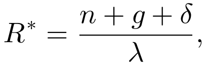
whatever the wage share. Four economies with wage shares from 0.2 to 0.8 all settle at R* = 2/15 (Figure 2).
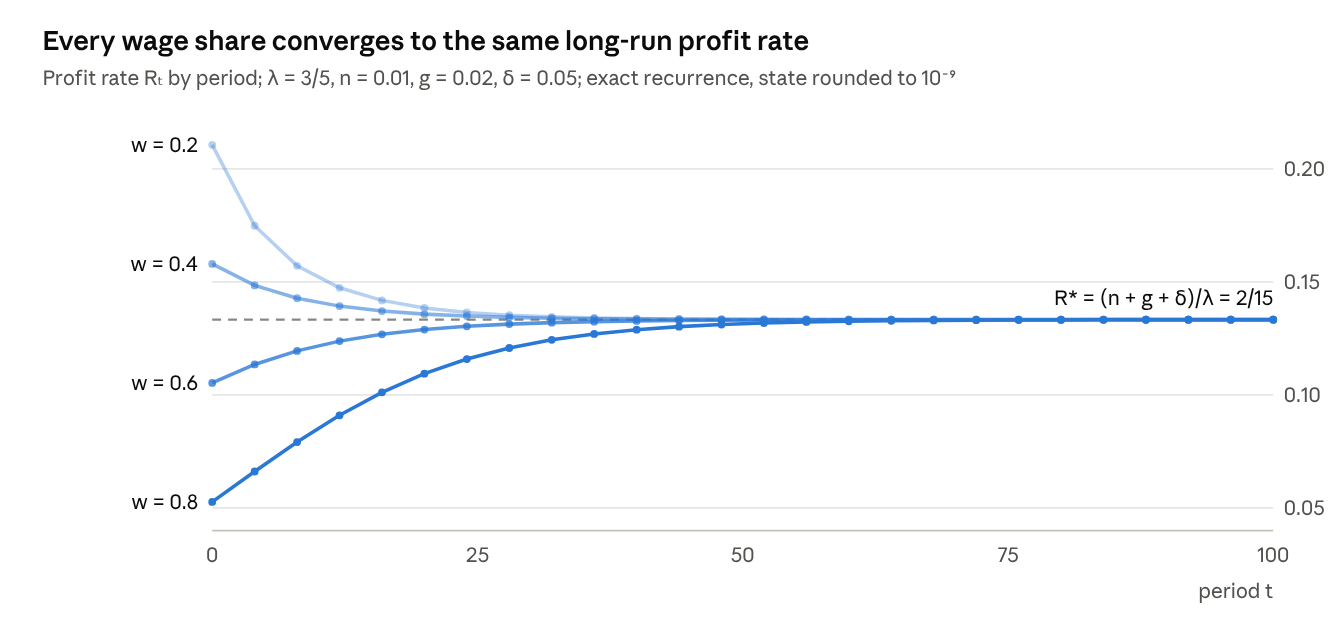
me-classical.pal §C1 every fourth period).The floor. Because there are always some workers per unit of capital (L/K > 0), the profit rate cannot fall below −(1 − w)(g + δ). The formula for R* leaves this floor out. The two meet when

| n | R* | floor | R after 599 periods |
|---|---|---|---|
| −0.0100 | 0.01667 | −0.00800 | 0.01667 |
| −0.0200 | 0 | −0.00800 | 0.00042 |
| −0.0248 | −0.00800 | −0.00800 | −0.00534 |
| −0.0300 | −0.01667 | −0.00800 | −0.00766 |
| −0.0500 | −0.05000 | −0.00800 | −0.00799 |
The rate actually reached is the larger of the two, max(R*, −(1 − w)(g + δ)). Near n* the approach slows to a crawl: after 599 periods at n = −0.0248 the rate is still 0.0027 above the floor, while at n = −0.05 it is within 10⁻⁵. Physicists call this critical slowing down, and it happens wherever two possible resting points swap stability. Cockshott is right that a shrinking population pushes the profit rate toward a negative level. The model adds three things: the rate has a lower bound, the bound depends on the wage share, and near the threshold the rate approaches it very slowly.
What the data say. Maito (2014) finds that the average profit rate of six core countries (Germany, the US, the Netherlands, Japan, the UK and Sweden) fell from 40.6% in 1870–1874 to 10.8% in 1982, then recovered to 14.6% in 2007. Basu (2022) finds a falling world trend for 1960–2019, driven by a falling ratio of output to capital. Holding exploitation constant matches Basu’s breakdown, and slowing population growth matches the long fall. The model reads the recovery of 1982–2007 as the counter-tendency of §8.3, a growing reserve army and a falling wage share.
Verdict: T5 is qualified by the model and supported by the data as a long-run tendency. It needs a rule for wages or slowing population growth.
5 Money and its distribution (T3, T4, T10)
If money is conserved when people trade, as energy is when molecules collide, then statistics alone decide how it ends up spread across a population, before anyone’s merit comes into it. Capital income and newly created money then distort that spread, and the planning proposal is meant to undo the distortions. The results here are checked by me-distribution.pal (18 assertions). Its random numbers come from a fixed formula, so every sample comes out the same on every computer.
5.1 Conservation and the exponential law (T3)
The model. Following Drăgulescu and Yakovenko (2000), suppose every way of dividing M units of money among N people is equally likely. Then the chance that one person holds k units is:

As N grows this approaches a geometric (exponential-like) law. The total-variation distance between the two, a standard measure of how different two distributions are, falls to 0.0003 at N = 1000. When the average holding is T = 10, the geometric ratio is q = T/(1 + T) = 10/11, and the Gini coefficient (0 for perfect equality, 1 for one person holding everything) is 1/(1 + q) = 11/21 ≈ 0.524.
The same law appears if you simply let people trade. In a simulation of 100 people exchanging one unit at random, the Gini rises from 0 to 0.46 after 20,000 trades, and 9.20% of people end up with nothing, against 9.09% predicted. Nobody in the simulation does anything except trade at random. So this much inequality needs no differences in productivity or effort; conservation is enough.
What the data say. Ludwig and Yakovenko (2022) find that the bottom 96% of US tax units follow an exponential law, with a Gini near 0.5, over 1983–2018. The model’s 0.524 is the version of that figure for whole units of money.
5.2 Capital income, condensation and the asset cap (T3, T10)
The model. Five owners and 95 workers trade in two kinds of event. A wage payment adds a fixed amount: an owner pays a random worker one unit. A sale works like interest: the owner who receives the payment is picked in proportion to how much each owner already has, so the rich are likelier to get richer. The planning post’s cap θ on private holdings is one more rule, which moves anything above the cap into a public fund that pays wages.
| cap θ | owners’ share after 60,000 events | workers’ Gini | owners’ holdings |
|---|---|---|---|
| none | 0.9764 | 0.8439 | (0, 0, 0, 0, 952) |
| 60 | 0.2421 | 0.4905 | (0, 58, 59, 59, 60) |
| 30 | 0.1159 | 0.4859 | (4, 25, 26, 29, 29) |
Without a cap, capital income does more than produce a Pareto tail, the long thin tail of very large fortunes. The money “condenses”: one owner ends up with 98% of all of it. With a cap, the owners’ share stays below Cθ/M (C owners, each capped at θ, out of M in total), and the workers’ Gini stays near 0.49.
What the data say. In Ludwig and Yakovenko (2022), the top 4% of incomes form a Pareto tail holding 34% of income in 2018. The Federal Reserve’s Distributional Financial Accounts put the top 1%’s share of wealth at 32.5% in the second quarter of 2026. So the model points the right way, but it overshoots badly. Real economies keep wealth to a power law through forces the model leaves out: returns that vary from fortune to fortune, taxes, bankruptcy, and fortunes divided among heirs. Section 9.2 adds them.
5.3 Money creation and labor vouchers (T4, T10)
Money creation. Take an economy that produces Q = 1000 units of goods, where three groups (asset holders, the middle, and the poor) hold 600, 300 and 100 units of money. Give 100 newly created units to the asset holders, and let them spend before prices adjust. In real terms the asset holders gain 100 units of goods, the middle loses 75 and the poor lose 25. The gains and losses add to zero, and the first recipients gain exactly Q·D/M, where D is the new money and M the old money supply. If instead the same new money is handed out in proportion to what people already hold, and spent after prices adjust, nobody gains or loses. Creating money does not create goods. It changes who gets to claim the goods that already exist.
What the data say. Domanski, Scatigna and Zabai (2016) find that after 2008, monetary policy widened wealth inequality mainly by raising share prices, which benefits people who own shares. That is the same mechanism, known after Richard Cantillon as the Cantillon effect: new money benefits whoever receives it first.
Vouchers. Labor vouchers are issued for hours worked and cancelled when they are spent. No rule in the model moves a voucher from one person to another. So one person’s extra work changes nobody else’s holdings, which is not true of money, and there is no rule that would let anyone use vouchers to make more vouchers.
Verdict: T3 is derived and supported for the lower class, and qualified for the upper class, whose concentration the model overstates. T4 is derived and supported in direction. T10 is derived.
6 Class conflict in the labor market (T8)
Up to now the wage has simply been given. This section works it out from class positions. What a worker can fall back on (the reserve army under capitalism, or the job guarantee under planning) decides the bargain. The bargain in turn decides what is at stake in a game where labor can organize and capital can give in, crack down, or leave. The results are checked by me-games.pal (20 assertions), with thresholds from me-extremes.pal (§X1–X2) and data from me-evidence.pal.
6.1 The reserve army as a fallback
The bargain. A worker bargains with power β, a number between 0 and 1. If bargaining fails, she finds another job with probability 1 − u, where u is the unemployment rate, and otherwise lives on a benefit s. Under a job guarantee paying g, the guarantee becomes her fallback instead. The standard Nash bargaining solution gives these wage shares:

Under capitalism the wage has two limits. At full employment, w(0) = 1: the threat of dismissal means nothing, because another job is always available, so labor takes the whole product. At total unemployment, w(1) = β + (1 − β)s = 13/25.
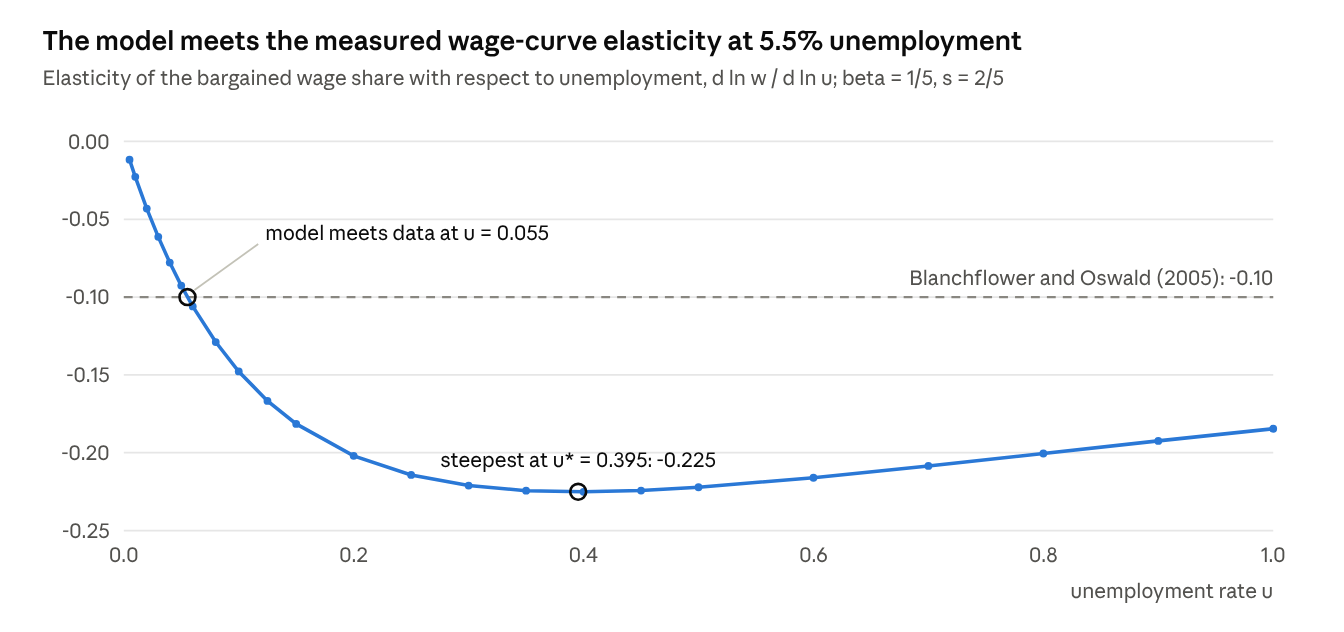
Where the wage reacts most. The elasticity of the wage with respect to unemployment says by what percentage the wage falls when unemployment rises by one percent. Here it is

which is zero at both ends. It is largest in size at

So the reserve army has the least power over wages near full employment and the most at about 40% unemployment.
What the data say. Blanchflower and Oswald (2005) estimate that pay responds to local unemployment with an elasticity of about −0.1, much the same across countries. The model gives −0.093 at 5% unemployment and −0.148 at 10%, and it passes −0.10 at 5.54% (Figure 3). I did not choose any parameter to get this. The model also makes a prediction that could be tested: the wage curve should flatten out when unemployment is low.
me-extremes.pal §X1).6.2 The class-struggle game and capital flight
The game. Workers either accept the terms or organize. Capital either gives in (concedes), cracks down (represses) at a cost ρ, or moves abroad (flees) and earns r_ext there. Organizing costs workers k and raises their bargaining power from b_l to b_h, unless capital represses. With b_l = 1/5, b_h = 1/2, k = ρ = 1/20, r_ext = 1/10, s = 2/5 and g = 4/5, at u = 1/5, the payoffs are:
| profile | capitalism: W | capitalism: C | planning: W | planning: C |
|---|---|---|---|---|
| accept / concede | 0.7333 | 0.2667 | 0.8400 | 0.1600 |
| accept / repress | 0.7333 | 0.2167 | 0.8400 | 0.0600 |
| accept / flee | 0.4000 | 0.1000 | 0.8000 | 0.0000 |
| organize / concede | 0.8500 | 0.1000 | 0.8500 | 0.1000 |
| organize / repress | 0.6833 | 0.2167 | 0.8500 | 0.0000 |
| organize / flee | 0.4000 | 0.1000 | 0.8000 | 0.0000 |
Under capitalism there is no pure Nash equilibrium, meaning no pair of choices that neither side wants to change. Instead the two sides keep switching, and the only stable outcome is a mixed one in which workers accept 70% of the time and capital concedes 30% of the time. Under planning, repression fails and flight triggers expropriation, so there is a single stable outcome: workers organize and capital concedes. I checked 243 combinations of the settings. Planning always has a stable outcome in which capital concedes; capitalism has none in 187 of them.
Along the unemployment axis. Under capitalism the game changes character at two points.
- When u ≤ 1/12 (0.0833), capital flight is a stable outcome. Up to u = 1/20 there are two such outcomes, (accept, flee) and (organize, flee); above it only (organize, flee) remains.
- When u > 1/12, there is no stable pure outcome. Labor’s average bargaining power falls from 0.2549 at u = 0.10 to 0.2188 at u = 0.50.
Michał Kalecki described this in 1943 as the political limit to full employment. Near full employment the wage takes nearly the whole product, so capital’s best response to organized labor is to leave. Section 9.7 lets the return abroad vary.
6.3 The job guarantee
A job guarantee raises private wages only if the guaranteed job pays better than what workers could get under the reserve army, w_ap > w_cap. Setting the two equal gives the point where that starts:

Below 9.1% unemployment the guarantee does nothing to private wages, because private employers already pay more than the guaranteed job. Above it, the gain rises: +1.4% at 10% unemployment, +5.0% at 12.5% and +14.5% at 20%.
What the data say. Imbert and Papp (2015) find that India’s NREGA, a rural employment guarantee, raised private rural wages by about 5%, while each public job replaced one private job. In a randomized rollout of better NREGA payments, Muralidharan, Niehaus and Sukhtankar (2023) find that 86% of the extra earnings came from outside the program, because private wages and employment both rose. The model gives +5% at 12.5% unemployment, a slack rural labor market, through exactly that channel: the guarantee improves the worker’s fallback.
Verdict: T8 is reproduced above 1/11 unemployment and supported in slack labor markets. At low unemployment the guarantee has no effect in the model, partly because of how the bargaining formula behaves near full employment (§12.1).
6.4 Exploitation as a property relation
John Roemer’s test calls a group of people exploited if they would be better off leaving with their per-head share of society’s capital and working it themselves. Six people hold capital (0, 0, 0, 1, 2, 9), and a job needs 4 units. On all 63 possible groups, the test agrees with a simple rule: a group is exploited when its average capital is below society’s average. When every worker has access to the social means of production, as under a job guarantee with land and job assignment, no group is exploited. Roemer’s thought experiment becomes an institution.
7 Politics (T7, T9, T11, T12)
The economy reaches politics through living standards. When they fall, voters weigh a radical gamble against a moderate sure thing. Networks that hand out jobs shape what voters expect. And the way a government is organized decides whether officials can collude against everyone else. This section builds each of these mechanisms on its own; §8 connects them to the economy. The results are checked by me-games.pal and me-selectorate.pal (7 assertions), with thresholds from me-extremes.pal (§X4, §X8–X9).
7.1 Losses, curvature and the radical coalition (T11)
The choice. Voters choose between a moderate option, a sure gain of +1, and a radical gamble that pays +6 with probability 1/4 and −2 with probability 3/4. The gamble’s expected value is 0, below the moderate option’s. Following Kahneman and Tversky’s prospect theory (1979), voters judge outcomes as gains or losses from where they stand, D, relative to what they consider normal. Losses hurt more than equal gains please, by the loss-aversion factor λ = 9/4 that Tversky and Kahneman (1992) estimated. I use a piecewise quadratic value function so that every calculation stays exact:

Voters pick the gamble exactly when D is below −5.399. The fascism post names four groups of people, two falling (by 6 and 3) and two rising (by 1 and 2). Weighted by size, 30% of them would choose the gamble. If each group measures itself against an aspiration 3 units above where it stands, 55% would. If every group is rising, as in the Cold War years, none would.
What sets the threshold. The fascism post puts radicalization down to loss aversion. When every possible outcome is a loss (D < −6), loss aversion multiplies both sides of the comparison equally and cancels out, and the condition becomes

| curvature K | 10 | 20 | 40 | 80 |
|---|---|---|---|---|
| threshold at λ = 9/4 | −5.399 | −14.5 | −34.5 | −74.5 |
| threshold at λ = 1 | −4.838 | −14.5 | −34.5 | −74.5 |
| 11/2 − K | −4.5 | −14.5 | −34.5 | −74.5 |
This holds exactly for K > 23/2. At K = 10 the threshold, −5.399, lies above −6, so it is not quite 11/2 − K. Raising loss aversion from 1 to 100 moves the threshold by only 0.74. Making the value function flatter (a larger K, which means people’s sensitivity to losses fades less as losses grow) moves it without limit, and a voter with a perfectly straight value function never takes the gamble. So what produces the radical coalition is how people’s sensitivity to losses changes as losses deepen, the convex shape that makes a gamble attractive to those already far behind. Loss aversion matters much less.
What the data say. Funke, Schularick and Trebesch (2016) find that far-right vote shares rise by about 30% after financial crises, across 1870–2014, but not after ordinary recessions. In the model, too, only a deep loss crosses the threshold. Lakner and Milanovic (2016) supply a related fact about who loses: in 1988–2008 the lower-middle class of rich countries saw almost no income growth. That is the group the fascism post describes as falling.
Verdict: T11 is qualified by the model and supported by the data. A radical coalition forms only past a threshold of loss, and the curvature of the value function sets it.
7.2 Patronage (T12)
The model. Two political networks, one left and one right, spend their resources on jobs and on messages. Following the job-creation post, a job ties a member to a network three times as strongly as a message does, and resources follow membership. If the right network is funded by capital (base funding 3 to 1), the best strategy for both networks, whatever the other does, is to spend everything on jobs. If the left creates no jobs while the right does, the right ends up with 0.942 of the membership, against 0.743 if both create jobs.
What the data say. Thachil (2011) shows that the BJP’s service networks in India win the votes of poor people who would otherwise oppose the party’s elite program. Material help ties people more strongly than messages do.
Verdict: T12’s premise is supported, and its conclusion is reproduced in this static setting. Whether patronage becomes a self-reinforcing spiral over time is a question about dynamics, which §8.4 takes up.
7.3 Collusion and the divided government (T9)
The model. K officials share a bribe, or rent, R if they all collude. Any one of them can blow the whistle and collect a reward B, and an audit uncovers the conspiracy with probability P each period. Collusion can last, with each official cooperating as long as everyone else does, only if they value the future enough. Their discount factor δ must be at least
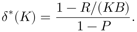
If the whistle-blower’s reward equals the rent (B = R), collusion fails for every discount factor once the number of independent officials reaches
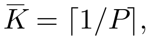
because δ*(K) ≥ 1 exactly when 1 − 1/K ≥ 1 − P. The program confirms this at five audit rates, from 5% (K̄ = 20) to 50% (K̄ = 2).
That gives the planning post’s divided government a design rule: it needs at least as many independently accountable offices as one over the chance of an audit. Fewer offices with more frequent audits work just as well. A single ruling party, whose members cannot collect a reward for reporting each other, can sustain collusion however little they value the future. That is Milovan Djilas’s “new class” (1957), here as the stable outcome of a game.
What the data say. Corporate leniency programs work the same way: they excuse the first member of a cartel who reports it. Miller (2009) finds that the US program, introduced in 1993, caught more cartels and discouraged new ones.
7.4 Political survival (T9)
Collusion is one way to hold power without being accountable. Selectorate theory describes another: a leader who needs only a few supporters can keep them loyal with private rewards.
The model. For the utility function the book uses, √x + √g + √y + √l, the model can be solved in closed form. The share of spending that goes on private rewards is
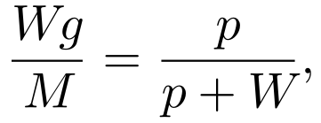
where W is the size of the winning coalition the leader depends on and p is the price of public goods. The book calls this “perhaps the key” result. As W grows, taxes, the private share and the leader’s surplus all fall.
How much the leader keeps depends on how much the coalition values the future (δ). With N = S = 100,000, W = 1,000 and p = 10,000:
| δ | incumbent tax | spending M | leader’s surplus | coalition member’s utility |
|---|---|---|---|---|
| 0 | 0.5619 | 17,117.7 | 0 | 5.538 |
| 0.5 | 0.5733 | 4,752.2 | 12,394.2 | 3.481 |
| 0.9 | 0.5832 | 207.6 | 16,949.3 | 1.668 |
| 0.99 | 0.5855 | 2.1 | 17,155.2 | 1.238 |
A coalition that cares nothing for the future (δ = 0) puts no value on loyalty, so the leader must spend all revenue to stay in power. A very patient coalition (δ close to 1) stays loyal almost for free, and the leader keeps nearly everything. Secure power breeds extraction. The selectorate model cannot tell accountable planning apart from any other majority-rule system, though, because it has no property relations and no division of offices. What makes the proposal distinctive lies outside this model.
Verdict: T9 is derived for collusion, with the design rule K̄ = ⌈ 1/P ⌉. Its selectorate reading is reproduced, but the evidence for selectorate theory is disputed (Clarke and Stone, 2008).
7.5 Quadratic voting and what gets produced (T7)
The model. In quadratic voting (QV; Lalley and Weyl, 2018), each voter has a budget of credits, and casting n votes on one issue costs n² credits. That lets people with strong feelings about one issue express them, at a rising price. Here 90 workers, 5 owners and 5 green voters spread their votes over investment, necessities and luxuries. The tally is (300, 450, 120), so luxuries get 13.8% of the votes. If instead demand is weighted by how much money people have, using the uncapped distribution of §5.2, 78.1% of spending goes on luxuries. In a market, purchasing power decides what gets made, not need.
Verdict: T7 is reproduced. Survey evidence on QV (Quarfoot et al., 2017) is consistent with it, but it is far from a test of QV as a way to plan production.
8 The whole economy (T11–T13)
The posts’ strongest claims are about how the mechanisms interact. Unemployment weakens labor, falling wages push voters into losses, a radical government represses unions, and patronage raises what people expect. This section runs all the mechanisms together, in three versions of the economy. The results are checked by me-regimes.pal (13 assertions), the self-rewriting me-economy.pal, me-loops.pal (5) and me-dialectics.pal (13).
8.1 One period as a chain of equations
Each period is a chain of equations, worked out in order over a record that holds the state of the economy. One equation connects the economy to the game of §6:
rule eq-B : (pe-eq B ?v ?p) => (pe-beta (pe-cs (@ ?v mode)) ?gp) where ?gp <- (pe-gpar ?v (put@ ?p u 0))
In words: each period, labor’s bargaining power is whatever the class-struggle game produces at that period’s unemployment rate. The chain then works out, in order:
- employment E = min(N, K/κ), where κ is the capital needed per job, rising by μ = 1% a period as work is mechanized;
- the wage share w, profit Π = (1 − w)E and the profit rate r = Π/K;
- investment I = s_c Π, or none at all (a capital strike) when the profit rate falls below a minimum, r_min, or when capital’s best move in the game is to flee;
- inflation and the living standard;
- the radical vote, measured against a reference point that the right network’s messaging pushes up;
- the right network’s share of membership;
- viability Φ = min(economic margin, 2(1/2 − radical vote)), a single number for whether the economy and its politics can carry on.
The three versions differ in their equations, not in their numbers:
| mechanism | capitalism | Cold War (to t = 30) | accountable planning |
|---|---|---|---|
| outside option | reserve army | plus insurance at 9/10 of the employed standard | job guarantee, g = 4/5 |
| wages | bargaining | floored to half of productivity growth | public wage; private firms must beat it |
| money | 2% inflation, 10% shock at t = 40–41 | the same, indexed | labor vouchers |
| left network | no jobs | jobs | jobs |
| repression | radical government halves bargaining power | the same | rights entrenched |
| capital | accumulates | accumulates | capped at θ = 60 |
The settings come from the model’s own steady-state algebra, not from fitting. Investment just keeps pace when s_c·r = δ + μ, so with s_c = 3/5, δ = 3% and μ = 1% the profit rate needed to keep going is r = 1/15.
8.2 Three versions of the economy
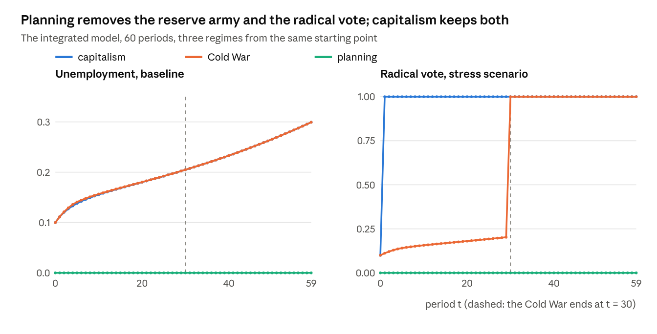
At the baseline settings (Figure 4):
- Capitalism. Unemployment rises in every period, from 0.100 to 0.299, and the wage share falls in every period.
- The Cold War. The radical vote is 0 until t = 30. After that the unemployed lose their insurance, and the radical vote equals the unemployment rate.
- Planning. Unemployment and the radical vote are 0, living standards rise, and Φ stays positive.
Under stress (an inflation shock, loss sensitivity 30 and aspiration messaging 0.40; see §8.4), capitalism elects a radical government that holds office for 58 of the 60 periods. The Cold War version does the same as soon as its concessions end. Planning never has a radical vote.
lib/polecon.pal).Labor’s share. The US Bureau of Labor Statistics reports that labor’s share of nonfarm business income fell from 66.2% in late 1960 to 52.8% in mid-2026, a relative fall of 20.2%. The model’s wage share under capitalism falls 19.9% over 60 periods, from 0.864 to 0.692, as mechanization weakens labor’s fallback. The levels differ, because the measured share counts employer contributions and treats depreciation differently; the match is in the size of the decline.
8.3 Unemployment and mechanization
Why does unemployment rise in every period? As long as there is no crisis and the economy is below full employment, capital and employment are tied together by

Employment holds steady only if μ = s_c·r − δ. Running capitalism at five rates of mechanization shows where that boundary lies:
| μ | u₀ | u₅₉ | r₅₉ | w₅₉ | μ that holds E constant at r₅₉ |
|---|---|---|---|---|---|
| 0 | 0.100 | 0.110 | 0.0500 | 0.850 | 0 |
| 0.005 | 0.100 | 0.179 | 0.0560 | 0.775 | 0.0036 |
| 0.010 | 0.100 | 0.299 | 0.0571 | 0.692 | 0.0042 |
| 0.015 | 0.100 | 0.461 | 0.0517 | 0.627 | 0.0010 |
| 0.020 | 0.100 | 0.596 | 0.0501 | 0.517 | 0.0001 |
Without mechanization the profit rate settles at δ/s_c = 0.05, and unemployment settles near 11%. With mechanization the profit rate never gets above about 0.057, so the fastest mechanization the economy can absorb is about 0.4% a period. Anything faster makes the reserve army grow forever. The table also shows that faster mechanization first raises the profit rate, by weakening labor, and then lowers it, because fewer workers produce less profit.
What the data say. Here the model fails. US unemployment (FRED, 1948–2026) has no long-run trend; it was 4.2% in September 2026. Barbosa-Filho and Taylor (2006) find the boom-and-squeeze cycles that Richard Goodwin described in US data. Real economies must sit close to the boundary μ ≈ s_c·r − δ, held there by things the model leaves out, such as demand management, the growth of services and shorter working hours. Section 9.6 adds two candidates, credit and mechanization that responds to wages.
8.4 Stress, lock-in and the tipping point (T11–T13)
Under stress (loss sensitivity 30, aspiration messaging 0.40), capitalism elects a radical government at t = 2. Repression halves labor’s bargaining power, and the profit rate jumps from 0.045 to 0.086. Living standards then rise from 0.85 to 2.10 by t = 45, yet the radical vote stays at 1.
The government stays because of the reference point. With the right network holding 85–89% of membership, every group compares itself with a standard 34–36% above its own, so it feels behind however much it gains. This is the job-creation post’s “downward spiral”, made precise.
How much does this depend on the settings? I ran a grid of 27 settings, varying loss sensitivity, the size of the inflation shock and aspiration messaging.
- Planning never has a radical vote after t = 1.
- The Cold War never does worse than capitalism.
- Capitalism elects a radical government in 15 of the 27.
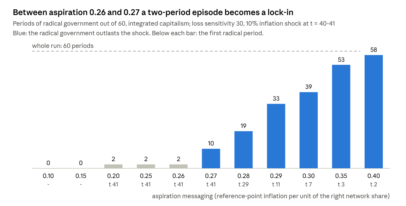
me-extremes.pal §X7).Where the spiral starts. Figure 5 varies aspiration messaging with the shock held fixed. Below 0.20 there is no radical government. From 0.20 to 0.26 the shock produces a two-period episode. At 0.27 the radical government outlasts the shock, for 10 periods. From 0.28 on it comes earlier and stays longer: 19 periods at 0.28, 39 at 0.30 and 58 of 60 at 0.40. The tipping point is sharp because the lock-in feeds itself: a radical government represses, profits rise, the right network grows on those profits, and aspirations rise with the network. Below the threshold the same shock produces only a protest vote that reverses, which matches what Funke and his coauthors find after ordinary recessions (§7.1).
Verdict: T11 and T12 are reproduced as dynamics above a threshold. T13 is reproduced in all 27 settings. No economy has run the planning proposal, so it cannot be tested against data.
8.5 Feedback loops
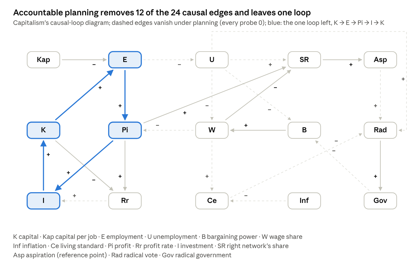
Put together, the mechanisms form a causal-loop diagram with 15 variables and 24 arrows, each marked as pushing its target up or down. The diagram has 14 loops: 5 reinforcing (they amplify a change) and 9 balancing (they damp it). Among them are the Goodwin profit squeeze (balancing), accumulation, radicalization and patronage (all reinforcing).
A diagram drawn by hand simply asserts its arrows. Here each arrow X → Y is checked against the equations themselves: raise X a little, freeze every other variable, recompute Y and read off which way it moved. I did this at ten different states of the economy, and 23 of the 24 arrows behave as drawn.
The exception is the arrow from unemployment to bargaining power, which turns positive near full employment. That is the capital-flight outcome of §6.2: where capital’s best answer to organized labor is to leave, more unemployment actually raises labor’s bargaining power. A hand-drawn diagram would have shown this arrow as negative everywhere.
Under planning, 12 arrows disappear: the reserve army, the trade-off between wages and profits, inflation, every route into the radical vote, and repression (Figure 6). One loop is left, accumulation in what remains of the private sector, and the asset cap limits it.
lib/polecon.pal, me-loops.pal §7.3).8.6 Structural dialectics applied to the model
The structural-dialectics post sets out tests for when a society should move to a new form. I applied them to the model for each period from t = 0 to 59. The diagnoses are s (stasis), I (instability), P (Phase Inversion) and n (not viable):
baseline capitalism ssssssssssssssssssssssssssssssssssssssssssssssssssssssssssssstress Cold War sssssssssssssssssssssssssssssIPnnnnnnnnnnnnnnnnnnnnnnnnnnnnnstress capitalism sPnnnnnnnnnnnnnnnnnnnnnnnnnnnnnnnnnnnnnnnnnnnnnnnnnnnnnnnnnnmoderate inflation crisis ssssssssssssssssssssssssssssssssssssssssPnssssssssssssssssss
Baseline capitalism stays in stasis throughout: rising unemployment alone does not justify a transition. The Cold War shows instability only in its last period, when its concessions end. A crisis opens a window of exactly one period before a radical government closes it, which is what the contradictions post calls foreclosure. Whether a transition would count as a synthesis depends on the reference point the new society inherits, which can make its first period not viable.
9 Finance (T14–T17)
In sections 4 to 8, money appears only as something conserved in trade and as a one-off injection of new money (§5.3). The posts say a good deal more about money, and the earlier version of this evaluation left it out. Four claims stand out.
- Credit money. The mechanical-materialism post says that when a bank makes a loan, it “does not lend out pre-existing deposits”, and that “New money bids up the price of housing and equities without a corresponding increase in the real output of the economy”.
- Capital gains. The same post traces the Pareto class, the small group of very large fortunes, to “compounding capital-gains income”, and says the class structure is not something that “could be reformed away with the right policies”.
- Debt deflation. The accountable-planning post says that “nearly all production is financed by borrowing”, and that falling prices start a spiral: “Falling prices cause insolvency, insolvency causes distress selling, distress selling causes further price declines”. So, it concludes, “The system requires that the purchasing power of money be deliberately eroded as a condition of its own stability”.
- Debt and desperation. The same post treats economic insecurity as “an existential threat in the same register as mortality”. The first version of this evaluation added, among its limitations: “Increasing debt increases desperation, and therefore the effects of Terror Management Theory.”
These become four new propositions:
| proposition | post (quoted) | tested in | |
|---|---|---|---|
| T14 | Credit creates money and inflates asset prices, not output | mechanical materialism: “New money bids up the price of housing and equities without a corresponding increase in the real output of the economy” | §9.1 |
| T15 | Compounding capital gains produce the Pareto class, which reform cannot remove | mechanical materialism: “The Pareto (superthermal) class corresponds to compounding capital-gains income” | §9.2 |
| T16 | Nominal debt makes deflation a self-reinforcing spiral, so the system needs inflation, which cuts real pay | accountable planning: “The system requires that the purchasing power of money be deliberately eroded as a condition of its own stability” | §9.3–9.4 |
| T17 | Debt deepens economic desperation and the turn to authoritarian options | accountable planning: insecurity is “an existential threat in the same register as mortality” | §9.5 |
Two other gaps in the first version also matter for earlier claims. Mechanization in the model was fixed in advance rather than chosen by firms, which the first version listed as a limitation; that bears on the unemployment failure of §8.3 (§9.6). And capital’s option to leave the country was held at a single fixed return abroad, which bears on the flight threshold of §6.2 (§9.7).
The results in this section are checked by me-finance.pal (7 assertions), me-financialized.pal (12) and the second table of me-evidence.pal (1). The independent cross-check adds 18 checks (§11).
9.1 Credit money and the price of houses (T14)
How banks create money. When a bank makes a loan, it does not hand over money someone else deposited. It credits the borrower’s account with a new deposit, and when the loan is repaid that deposit disappears. The model keeps a ledger of eight loans, payments and repayments, and after every one, the new deposits equal the loans still outstanding.
What credit does to prices. Now suppose buyers who have saved S each bid for a fixed stock of houses, and a bank will lend them a share LTV of the price (the loan-to-value ratio). A buyer can pay at most her savings plus the loan, S + LTV·P, and when buyers compete, the price rises to that limit. So
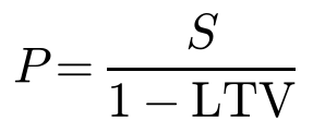
Raising LTV from 0 to 0.8 multiplies the price by 5. Raising it to 0.95 multiplies it by 20. Not a single house is built, and nothing else is produced either.
Each sale creates new money, the loan LTV·P, and pays it straight to the person who already owned the house. When the seller spends it, prices have not yet adjusted, so the seller gains exactly Q·D/M in real goods, the first-recipient gain of §5.3, and everyone else loses the same amount between them. At LTV = 0.95, ten sales a period move 190 of the economy’s 1,000 units of output to the sellers.
What the data say. Favara and Imbs (2015) study US bank-branching deregulation in 1994–2005, which let banks lend more for reasons unrelated to the housing market. The extra mortgage credit raised house prices. Only where it was easy to build did the number of houses grow instead. Jordà, Schularick and Taylor (2016) find that across 17 rich economies, mortgages rose from about 30% of bank lending in 1900 to about 60% today, and that nearly all of the financial sector’s growth since 1913 is mortgage lending to households, which “has little to do with the financing of the business sector”.
Verdict: T14 is derived, since the price formula and the transfer are accounting identities, and it is supported by the data.
9.2 Capital gains, resets and the Pareto class (T15)
In §5.2, capital income did more than create a class of large fortunes: all the money ended up with one owner. What that model lacked were the forces that break fortunes up.
The model. I call the simplest exact version a wealth lattice. Picture fortunes sitting on the rungs of a ladder, where each rung is worth twice the one below (levels 2ⁿ). Each period:
- a fortune moves up a rung (doubles) with probability p, which stands for a capital gain;
- it moves down a rung (halves) with probability q, which stands for a reset, such as division between two heirs, a bankruptcy or a tax;
- a fortune on the bottom rung, n = 0, has rejoined the ordinary exponential class and cannot fall further.
Over time the share of fortunes on each rung settles down to π_n = (1 − z)zⁿ, where z = p/q is how often fortunes double compared with how often they halve. The chance that a fortune is at least 2ⁿ is then

which is a Pareto law, the classic shape of the top of the wealth distribution. The single number α, the Pareto exponent, describes how heavy the tail is: the smaller α, the more the top fortunes dominate.
What happens next depends on whether fortunes are broken up often enough.
- If resets are frequent enough (z < 1/2, so α > 1), average wealth stays finite and every top share settles at a fixed value. Started with every fortune on the bottom rung, a ladder of 31 rungs reaches the settled distribution to within 10⁻⁶ in 300 periods.
- If resets are too rare (z ≥ 1/2, so α ≤ 1), average wealth grows without bound, and an ever smaller group ends up with nearly everything. With the ladder capped at rung L and z = 3/5, the top 1% hold 42.3%, 90.7%, 99.8% and 100.0% as L rises from 10 to 80. At z = 2/5, by contrast, their share settles at 32.5%.
The model of §5.2 is the case q = 0: no resets, so the money condenses into one fortune. The asset cap is a ladder with a top rung, so it limits the top share whatever z is.
The top 1%’s share changes quickly with α: 9.5% at α = 2, 17.9% at 1.58, 32.5% at 1.32 and 72.6% at 1.07 (Figure 7).
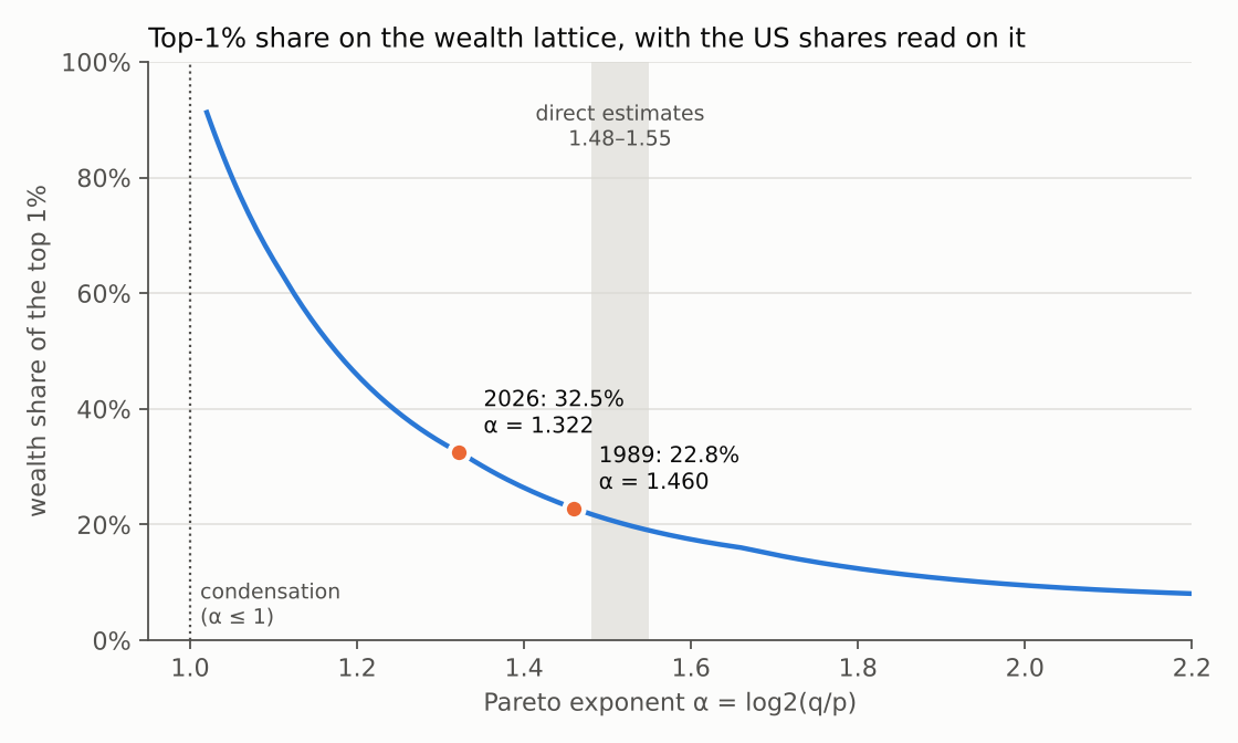
me-finance.pal §F2).What the data say. If I read the Federal Reserve’s figures for the top 1%’s share of wealth on this ladder, they imply α = 1.460 in 1989, when the share was 22.8%, and α = 1.322 in 2026, when it was 32.5%. The 1989 value is close to direct estimates of the US wealth tail: Klass et al. (2006) find 1.49 from the Forbes 400 for 1988–2003, and Vermeulen (2018) finds 1.48–1.55 after correcting for rich households that do not answer surveys. Benhabib and Bisin (2018) report both.
The rise in concentration since 1989 corresponds to a 10.1% rise in how often fortunes double compared with how often they are broken up. That has moved the tail about a third of the way toward α = 1, the point where wealth starts to condense. The ladder treats all fortunes as one Pareto population, so these numbers are a way of reading the data, not a fitted estimate.
Verdict: The first half of T15 is derived. Capital gains set against resets produce a Pareto class, with exponent log₂(q/p).
The second half, that the class cannot be reformed away, is qualified. The class itself is structural: any p > 0 and q > 0 produce a power law. Its size is not. The resets are inheritance rules, bankruptcy law and taxes, and between α = 2 and α = 1.07 the top 1%’s share changes almost eightfold. Reform cannot remove the class, but it decides how big the class is. The condensation that went wrong in §5.2 becomes a threshold, z = 1/2, and real economies sit below it.
9.3 Debt deflation (T16)
The model. Twenty firms each own one unit of an asset and owe debts d_j, spread evenly (a gap of Δ between one firm’s debt and the next) from d_lo to d_hi.
- A shock σ lowers the asset’s price to 1 − σ.
- A firm whose debt is larger than the price is insolvent, and it sells its asset.
- Each forced sale pushes the price down by η.
The model finds how many firms end up selling by repeating the count, firms whose debt exceeds the current price, until it stops changing. It also checks a formula against all 36 cases:
- if η ≥ Δ, one insolvency brings down every firm;
- if η < Δ, the sales stop after
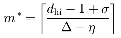
In plain terms, the spiral feeds itself when one forced sale pushes the price down by more than the gap to the next firm’s debt. Financialization narrows that gap, by crowding firms toward high levels of debt. With η = 0.025:
- firms whose debts are spread over [0.20, 0.80] (Δ = 0.032) absorb shocks of up to 20% without a single forced sale, and a 25% shock is amplified only 1.8 times;
- firms crowded into [0.50, 0.95] (Δ = 0.024) all collapse after a 10% shock, which is amplified six times.
What the data say. Irving Fisher (1933) laid out the chain from paying down debt to forced selling, falling prices, falling net worth and bankruptcy. He also stated its paradox: “Each dollar of debt still unpaid becomes a bigger dollar”, so that “the very effort of individuals to lessen their burden of debts increases it” (p. 344, as quoted by Shiller). The model reproduces this mechanism and its threshold. I have not compared it with Fisher’s numbers.
Verdict: The spiral in T16 is derived, with a threshold: it feeds itself only when forced sales move the price by more than the spacing of debts. Section 9.4 tests the second half of T16, the need for inflation, in the full economy.
9.4 Financialized capitalism (T16, T5)
The model. lib/polecon-fin.pal adds a fourth version of the economy to the three in §8. It is capitalism with three financial channels added, each one equation with one setting.
- Firms borrow to invest.
- Firms invest enough, (μ + δ)K, to keep their workforce as each job needs more capital. Banks lend a share lev of whatever their retained profit does not cover.
- Interest of 5% on firm debt comes out of profit, and the capital strike of §8.1 now looks at the profit rate after interest. So a debt crisis is the same crisis rule as before, reached through interest payments. This is the “Minsky moment”, named after Hyman Minsky, who argued that long booms financed by debt end this way.
- Debts are fixed in money, so inflation shrinks them in real terms. A crisis writes off the share of debt that the crash destroys, and banks stop lending.
- Households borrow to keep up.
- Employed households borrow half the gap between their aspiration (the reference point of §8.4) and their income after interest.
- Their debt is capped at one period’s income.
- In a crisis, lending stops and they must repay a fifth of what they owe.
- Debt adds to desperation.
- Debt payments are due whatever happens, so they come off what a worker can fall back on in the wage bargain. An indebted worker bargains from a weaker position.
- The share of income going on debt payments, DS, is added to unemployment as a source of insecurity, which strengthens the pull of the right network’s institutions. In the equation of §8.1, the terror-management term 3(1 + U) becomes 3(1 + U + DS).
- The interest households pay is income for capital, and it funds the right network along with profits.
With both kinds of borrowing switched off, this version reproduces capitalism period for period, and the program checks that it does.
The baseline run (lev = 1; Figure 8).
There are two crises, at t = 7 and t = 52, and each is followed by one period of radical government. Capitalism with the same settings has none.
Unemployment no longer rises every period. It stays flat between the crises, at 0.189–0.190 from t = 15 to t = 51, and jumps at each crisis. After 60 periods it is 0.298, against capitalism’s 0.299. Credit changes the shape of the rise, not its size.
Between the crises the wage share stays within 0.009 of a fixed level, while the profit rate falls every single period, from 0.073 to 0.040. Keeping people employed with borrowed money keeps the rate of exploitation constant, and as each job needs more capital, the profit rate falls. This is exactly the case §4.3 found when it held exploitation constant. There I had to assume it; here the economy produces it. The crisis then restores the profit rate.
Firm debt rises from 6.2% of capital at t = 24 to 19.0% at t = 51, as profits fall. Household debt sits at its ceiling from t = 15 until the inflation shock of t = 40–41 cuts real incomes.
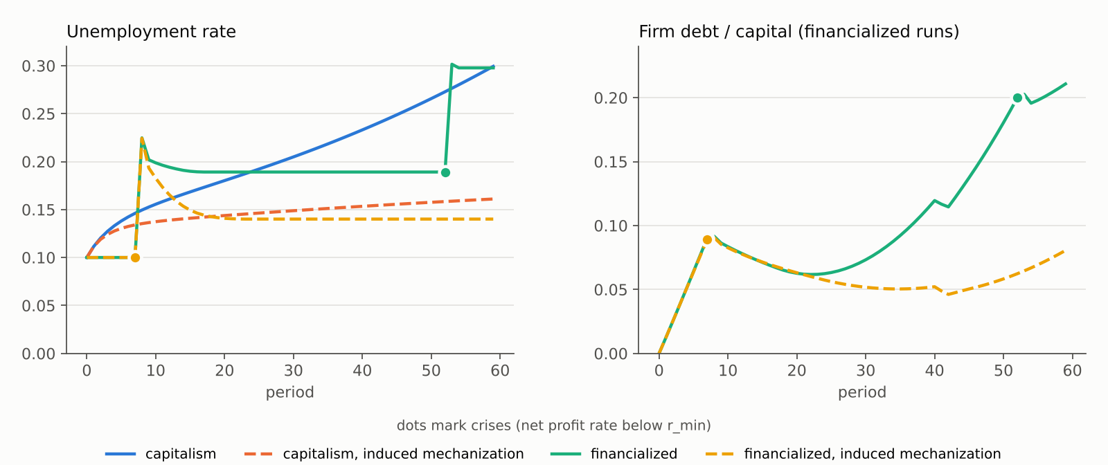
me-financialized.pal §F5.7, §F5.1).One channel at a time. Firm borrowing alone produces crises at t = 5 and 50 but no radical government. Household borrowing alone produces no crisis. Both together produce crises at t = 7 and 52, and each is followed by a radical government.
Where the behavior changes. How far the banks are willing to lend decides whether there is a crisis at all. When banks cover at most three-quarters of the gap (lev ≤ 3/4), there is no crisis within 60 periods, and unemployment ends lower than under capitalism (0.240 at lev = 3/4). The boundary lies between lev = 0.7617 and 0.7622.
Inflation delays the debt crisis but cannot prevent it. The first crisis (t = 6–8) comes from the falling profit rate and happens at every inflation rate I tried. The second comes later as inflation rises:
| steady inflation | 0 | 2% | 4% | 6% | 8% | 10% |
|---|---|---|---|---|---|---|
| second crisis | t = 48 | 52 | 54 | 57 | 59 | none in 60 periods |
| real pay cut between settlements, π/(1 + π) | 0 | 2.0% | 3.8% | 5.7% | 7.4% | 9.1% |
Deflation does the opposite. A 10% fall in prices at t = 40–41 raises the living standard of employed workers in debt-free capitalism, from 1.787 to 2.184, because their pay buys more. In the financialized economy the same fall in prices makes debts heavier. It lifts household debt above its ceiling, to 1.235 of income at t = 42, brings the second crisis forward from t = 52 to t = 49, and doubles the number of periods of radical government, from 2 to 4.
What the data say. US household debt rose to 99.1% of GDP in the first quarter of 2008 and has since fallen to 66.6% (first quarter of 2026; BIS data via FRED). That is the model’s pattern of debt rising to a ceiling and then being paid down, although the ceiling in the model is a chosen setting, not an estimate.
Verdict: T16 is reproduced and qualified. The financialized economy needs inflation to delay its debt crises, and the inflation that does so cuts real pay, as the post says. But inflation does not remove the crisis. It pushes the second one back by about one period for each percentage point.
T5 is reproduced in the financialized economy: credit supplies the rule for wages that §4.3 found the falling profit rate needs.
9.5 Debt, desperation and the radical vote (T17)
In §8.4 a shock turned into a radical government only under stress. In the financialized economy every crisis does so, even at the baseline settings. The reason is the credit crunch.
The crunch. In a crisis, banks stop lending and households start repaying, so employed workers’ living standard falls from a level that borrowing had propped up. That propped-up level is also what they had come to measure themselves against. The employed vote radical when their living standard falls below 1 + D*/20 = 0.730 of their aspiration, where D* = −5.399 is the threshold from §7.1.
| run | crisis | standard before | standard at crisis | change | standard / aspiration | radical |
|---|---|---|---|---|---|---|
| financialized | t = 7 | 1.095 | 0.851 | −22.3% | 0.670 | yes |
| financialized | t = 52 | 2.586 | 2.026 | −21.7% | 0.664 | yes |
| firm credit only | t = 5 | 0.935 | 0.959 | +2.5% | 0.889 | no |
| firm credit only | t = 50 | 2.491 | 2.553 | +2.5% | 0.871 | no |
Without household debt, the employed are slightly better off at the same crisis. In both runs, the program checks that each crisis produces a radical vote exactly when the ratio falls below 0.730. So a crisis becomes a radical government through the credit crunch, not through lost output: the crash destroys 10% of capital in both runs.
How much households borrow matters. If households borrow an eighth of the gap, neither crisis radicalizes voters. At a quarter or three-eighths, only the second does, after their debt has reached its ceiling. From a half upward, both do.
How much does this depend on the settings? Across the 27 stress settings of §8.4, capitalism elects a radical government in 15, and the financialized economy in all 27. Radical periods add up to 386 under capitalism and 509 with finance. In five settings finance actually shortens radical rule. All five are settings where capitalism is already locked in for 56 periods or more, and there borrowing lets households soften the blow.
The terror-management link. Three new arrows in the causal diagram hold with the expected sign at all ten states I checked: debt payments strengthen the right network (DS → SR), more debt means higher debt payments, and more debt lowers the wage, because the indebted worker bargains from a weaker position. The first link is weak, though. A rise of 0.05 in the debt-payment share raises the network’s share by only 0.001–0.004.
Through these arrows, finance adds two reinforcing loops of four links each:
- aspiration → household debt → debt payments → right network → aspiration;
- wage → right network → aspiration → debt → wage.
Firm debt adds a balancing loop, capital → debt → profit rate → investment → capital: debt brings on the crisis that writes it off. The financialized diagram has 36 arrows and 37 loops, and 18 of the loops pass through a financial variable (7 reinforcing, 11 balancing).
Two arrows fail their checks. The arrow from unemployment to bargaining power fails, as it did in §8.5. And the arrow from inflation to household debt, which I expected to be negative because inflation shrinks debt, turns out positive at the first state checked, where households owe little. There, inflation cuts real pay, and households borrow to make up the difference. Which effect wins depends on how much they already owe.
What the data say.
- Funke, Schularick and Trebesch (2016) find that far-right vote shares rise by about 30% after financial crises but not after ordinary recessions. The crunch in the model produces the same pattern.
- Mian, Sufi and Trebbi (2014) find that countries become more politically polarized and fragmented after financial crises.
- Mian, Rao and Sufi (2013) find that in the 2006–09 housing collapse, spending responded most to lost wealth in ZIP codes where households were poorer and more indebted, and spent more of each dollar of housing wealth.
- Jordà, Schularick and Taylor (2013) find that recessions with a financial crisis cost more output. Three years after the peak, real GDP per person is 2.5% below it after a financial crisis, and 2.0% above it after a normal recession. The model does not reproduce this: its crises destroy the same capital whether or not households are in debt.
Verdict: T17 is reproduced, and the data support its political pattern. In the model, debt drives people to radical politics mainly through the fall from a living standard that borrowing had inflated, and only weakly through the burden of debt payments. That adds to the finding of §7.1: financial crises cross the threshold of loss because credit has raised the standard people compare themselves with, and the crunch then takes it away.
9.6 Two possible fixes for rising unemployment
Section 8.3 found the model’s clearest failure against the data: unemployment rises without limit, while US unemployment has no trend. Two mechanisms the first version left out could hold it down. Credit is one (§9.4).
The other is the loop that §4.3 closed only on paper: firms mechanize when labor is expensive and hold back when it is cheap. I let capital per job rise at
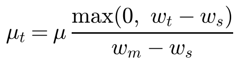
So mechanization runs at the full 1% a period when the wage share is at its starting level, w_m = 0.864, and stops at w_s = 0.765, a wage share lower by 1.129, the switch ratio found in §4.3.
| run | u₀ | u₁₅ | u₃₀ | u₄₅ | u₅₉ | wage share, 60 periods | r₅₉ | crises |
|---|---|---|---|---|---|---|---|---|
| capitalism | 0.100 | 0.168 | 0.205 | 0.249 | 0.299 | −19.9% | 0.0571 | none |
| capitalism, induced | 0.100 | 0.141 | 0.149 | 0.156 | 0.161 | −8.4% | 0.0538 | none |
| financialized | 0.100 | 0.190 | 0.189 | 0.189 | 0.298 | −21.7% | 0.0494 | t = 7, 52 |
| financialized, induced | 0.100 | 0.149 | 0.140 | 0.140 | 0.140 | −7.2% | 0.0477 | t = 7 |
Wage-driven mechanization stops the rise. After t = 30, unemployment rises by less than 0.001 a period. With credit as well, it stays at 0.140 in every period from t = 30, after a single crisis. The switch share w_s sets where unemployment levels off: at 0.187 when w_s = 0.70, and at 0.117 when w_s = 0.84.
But the fix costs the model its best match with the data. Labor’s share now falls only 8.4% (7.2% with credit), against 20.2% in the data. Across the different switch shares, the less unemployment rises, the less labor’s share falls: from −11.2% when unemployment ends at 0.187, down to −2.7% when it ends at 0.117.
The reason is that in this model, labor’s share depends on unemployment, and debt (§9.4) shifts it by only a point or two. So the earlier match in §8.2, a fall of 19.9% against 20.2% in the data, is the same fact as the unemployment failure. The US combination, labor’s share down by a fifth with no rise in unemployment, needs labor’s bargaining power to fall at any given level of unemployment, and neither fix provides that.
9.7 Capital mobility and Kalecki’s threshold (T8)
Capital’s freedom to move abroad is one candidate for that fall. In §6.2 the return abroad, r_ext, was fixed at 10%. Moving abroad becomes one of capital’s best options when the wage bargained against the reserve army reaches 1 − ρ − r_ext. For returns between 5% and 40%, that means

The game and the formula agree at all seven returns I tested. (At a return of zero the formula does not apply: flight is then a best option only at full employment.)
| return abroad | 5% | 10% | 15% | 20% | 25% | 30% | 40% |
|---|---|---|---|---|---|---|---|
| flight up to unemployment u_f | 5.0% | 8.3% | 12.5% | 17.9% | 25.0% | 35.0% | 75.0% |
From r_ext = 43%, flight is a best option at every level of unemployment. So easier movement of capital raises the unemployment rate below which capital leaves. It also lowers, point for point, the highest wage share at which capital stays and invests at home: from 0.85 to 0.80 as r_ext rises from 10% to 15%.
What the data say. Furceri, Loungani and Ostry (2019) find that when countries open their capital accounts, labor’s share falls by about 4.5% over the following years, most in industries that rely on outside finance.
The model’s version of this is cruder. When the game has no stable pure outcome, the return abroad does not enter the mixed one, so openness moves the flight threshold but not the bargained wage. On its own it cannot explain the combination described in §9.6.
Under planning, an attempt to flee triggers expropriation, so capital mobility leaves the job guarantee of T8 untouched. Under capitalism, Kalecki’s political limit to full employment moves with financial openness.
10 Assessment
10.1 The scorecard
The table collects the verdicts of sections 4 to 9.
| proposition | model | data | limit or condition | § | |
|---|---|---|---|---|---|
| T1 | value conserved in exchange | derived | not directly testable | holds for any transitive exchange table, fails for any intransitive one | 4.1 |
| T2 | values predict prices | derived, deviation growing in r | supported (r ≈ 0.94–0.99) | deviations 3–11× too small in a 3–4-sector model | 4.2 |
| T3 | exponential lower class, Pareto upper class | lower class derived; upper class qualified, and derived once fortunes can be broken up (§9.2) | lower class supported (Gini 0.5); upper class matched by the lattice reading (α = 1.46 vs 1.48–1.55) | condensation without resets (98% to one owner), a Pareto tail with them (z < 1/2) | 5.1–5.2, 9.2 |
| T4 | money creation redistributes | derived (zero-sum; first recipients gain Q·D/M) | supported (BIS) | a proportional injection spent after prices adjust redistributes nothing | 5.3 |
| T5 | falling profit rate | qualified: needs a wage rule or slowing demography; reproduced under financialization (§9.4) | supported as a long-run trend (Maito, Basu) | floor −(1 − w)(g + δ) below n* = −0.0248, with slow convergence there | 4.3, 8.3 |
| T6 | planning converges fast | derived (18 passes) | consistent with the post’s worked example | speed set by the spectral radius of A | 4.1 |
| T7 | QV redirects production toward need | reproduced | weakly supported (survey QV) | none found | 7.5 |
| T8 | job guarantee breaks employer power | reproduced above u_c = 1/11 | supported in slack markets (NREGA) | inert below 9.1% unemployment; capital flight up to u_f, which rises with the return abroad | 6.1–6.3, 9.7 |
| T9 | divided government cannot conspire | derived: K̄ = ⌈ 1/P ⌉ | plausible (leniency programs); selectorate evidence contested | a single party sustains collusion at every δ | 7.3–7.4 |
| T10 | vouchers and caps prevent accumulation | derived (non-interference; bounded owners’ share) | no test available | the cap bounds the last reinforcing loop | 5.2–5.3, 8.5 |
| T11 | losses and inflation drive radicalism | qualified: requires D < −5.4, a curvature effect | supported and qualified (crises, not ordinary recessions) | threshold 11/2 − K in deep losses; tipping point at aspiration 0.26–0.27 | 7.1, 8.2, 8.4 |
| T12 | patronage spiral | reproduced | premise supported (Thachil) | a spiral only above a threshold; below it the protest vote reverses | 7.2, 8.4 |
| T13 | planning defuses authoritarianism | reproduced in all 27 stress settings | no test available | an inherited reference point can make the successor’s first period non-viable | 8.4–8.6 |
| T14 | credit inflates asset prices, not output | derived (P = S/(1 − LTV); the sellers gain Q·D/M) | supported (Favara and Imbs; mortgages 30% → 60% of bank lending) | none: accounting identities | 9.1 |
| T15 | capital gains make the Pareto class, which reform cannot remove | derived (α = log₂(q/p)); “cannot be reformed away” qualified | supported (lattice reading 1.46 in 1989; direct estimates 1.48–1.55) | condensation iff 2p ≥ q; the exponent is set by resets, which are policy | 9.2 |
| T16 | debt deflation; the system needs inflation | spiral derived with a threshold; the need for inflation reproduced as postponement | supported (Fisher 1933) | complete spiral iff η ≥ Δ; second crisis at t = 48 → 59 for π = 0 → 8% | 9.3–9.4 |
| T17 | debt deepens desperation and radicalism | reproduced (2 of 2 crises radical with household credit, 0 of 2 without; 27 of 27 stress settings) | supported (Funke et al.; Mian, Sufi and Trebbi; Mian, Rao and Sufi) | standard/aspiration < 0.730 at the crunch; deeper output losses not reproduced | 9.5 |
10.2 The data at a glance
examples/me-evidence.pal prints the model’s figures next to the data, with the financial comparisons in a second table (§EV2):
§EV THE MODEL AGAINST EMPIRICAL DATA quantity data model wage-curve elasticity at u = 5% / 10% -0.10 -0.093 / -0.148 ... unemployment at which the model gives -0.10: 0.0554 labor share, relative change -20.2% -19.9% (60 periods) ... levels: data 66.2% -> 52.8%; model 0.864 -> 0.692 price-value MAWD 9.2% E3 at r*: 0.8%; CE Table 10.1: 3.1% job-guarantee wage effect +5.0% +1.4% / +8.4% / +14.5% at u = 10/15/20% ... no effect below u_c = 1/11; +5% at u = 0.1250 Gini of the exponential (lower) class 0.500 0.524 (geometric law, T = 10) loss aversion lambda 2.25 2.25 (input; the threshold moves by 0.18 from lambda = 2 to 10, me-extremes §X4)§EV2 FINANCE: THE MODEL AGAINST EMPIRICAL DATA quantity data model Pareto exponent of US wealth 1.49 1.460 (the lattice reading of the 1989 top-1% share) ... top-1% share 22.8% -> 32.5% (1989 -> 2026): alpha 1.460 -> 1.322; condensation at 1 far-right vote after financial crises +30.0% radical government after 2 of 2 crunches with household debt, 0 of 2 without ... the employed standard in the crunch: -22.3% / -21.7% with household debt; +2.5% without labor share, relative change -20.2% financialized -21.7%; induced mechanization -8.4% (u_59 0.161) capital-account opening, labor share -4.5% wage-share ceiling 1 - rho - r_ext: -5.9% (r_ext 10% -> 15%)
10.3 Five patterns
- The core holds. Conservation, the trade-off between wages and profits, the reserve army’s pull on wages and the exponential lower class all follow from the rules.
- Unconditional claims turn out to have conditions. The radical vote needs D < −5.4, the job guarantee needs u > 1/11, and a falling profit rate needs μ > s_c·r − δ or n < n*. Where data exist, they agree with the conditions: radicalization follows financial crises and not ordinary recessions, and the job guarantee’s effect on wages shows up in slack labor markets.
- The misses are about size, not direction. In the first version, three sizes were wrong. Prices stray from values too little, wealth concentrates too much, and unemployment rises without limit. In each case the model pointed the right way and something was missing: industry detail, the forces that keep wealth to a power law, and demand. Section 9 supplies two of the missing pieces. Breaking up fortunes turns condensation into a Pareto tail, and reading the 1989 top-1% share that way gives an exponent of 1.46, close to the measured 1.48–1.55. Wage-driven mechanization stops unemployment rising, but it shows that the labor-share match depended on that rise.
- Finance strengthens the political mechanisms. Every financial crisis in the model becomes a radical government, through the credit crunch that takes away a living standard borrowing had propped up. That matches what Funke and his coauthors find: radicalization after financial crises, not after ordinary recessions.
- Some claims are beyond the data. In the model, vouchers, the asset cap and a divided government remove the mechanisms the posts blame. No economy has tried them, so whether they would work as modeled cannot be tested.
11 Checking and reproducing the results
Every result is checked twice: by the assertions in the program that computes it, and by a separate Python program that recomputes every table from scratch and compares the text character for character.
All you need is a Rust toolchain (cargo) and Python 3:
cargo build --releasecargo test --release # 44 unit tests, among them exact arithmetic, memo, trace./verify-materialist.sh # 15 checks, about 6 minutes; exit status 0 iff all pass# individual programs (--dry-run: never write files)./target/release/palimpsest examples/me-tour.pal --trace 22./target/release/palimpsest examples/me-value.pal --dry-run # 7 s, 17 assertions./target/release/palimpsest examples/me-classical.pal --dry-run # 7 s, 8 assertions./target/release/palimpsest examples/me-distribution.pal --dry-run # 76 s, 18 assertions./target/release/palimpsest examples/me-games.pal --dry-run # 8 s, 20 assertions./target/release/palimpsest examples/me-selectorate.pal --dry-run # 9 s, 7 assertions./target/release/palimpsest examples/me-regimes.pal --dry-run # 84 s, 13 assertions./target/release/palimpsest examples/me-loops.pal --dry-run # 16 s, 5 assertions./target/release/palimpsest examples/me-dialectics.pal --dry-run # 5 s, 13 assertions./target/release/palimpsest examples/me-extremes.pal --dry-run # 11 s, 6 assertions./target/release/palimpsest examples/me-evidence.pal --dry-run # 2 s, 4 assertions./target/release/palimpsest examples/me-finance.pal --dry-run # 19 s, 7 assertions./target/release/palimpsest examples/me-financialized.pal --dry-run # 56 s, 12 assertions# the self-rewriting economy: run on a copy; six runs rewrite it, the seventh is a fixed pointcp examples/me-economy.pal /tmp/e.pal && sed -i 's#import "../lib/#import "#' /tmp/e.palfor i in 1 2 3 4 5 6 7; do PALIMPSEST_LIB=$PWD/lib ./target/release/palimpsest /tmp/e.pal | grep -E 'WROTE|FIXED POINT'; donepython3 crosscheck/materialist_crosscheck.py # 80 independent checks
The same programs run, more slowly, in the Palimpsest playground, with the same output and step counts.
Two implementations that share a specification but no code catch programming mistakes: a period off by one, a wrong rounding, a sign flipped in a probe, a payoff copied wrongly. They cannot catch a mistake in the specification itself. That is what the comparisons with data are for.
12 Limitations
12.1 The model
- It formalizes; it does not estimate. The settings come from the model’s own steady-state algebra or from the posts. A match without fitting is evidence that a mechanism works, not evidence that the model is calibrated.
- The bargaining formula lets labor’s share approach 1 at full employment. That drives capital flight below 1/12 unemployment (§6.2) and the job guarantee’s lack of effect below 1/11 (§6.3). A formula with a ceiling set by productivity, or a floor from efficiency wages, would move both thresholds.
- Mechanization is fixed in advance in the three versions of §8. Capital per job grows at a constant rate μ. Section 9.6 lets firms choose it, as an option; unemployment then stops rising, but the labor-share match goes.
- There is no demand side. Output is whatever the employed produce. Credit (§9.4) pays for investment and consumption, and debt now adds to desperation and the terror-management link, but nothing in the model captures a crisis of unsold goods or government spending.
- The financial settings are round numbers, not derived values. They are the interest rate (5%), how much of the gap banks lend (lev = 1), how much households borrow (half the gap), the debt ceiling (one period’s income) and the repayment in a crunch (a fifth). For each one that changes an outcome, §9 shows a range of values and the point where the outcome changes.
- The financial model is partial. Households never default, the unemployed carry no debt, and the interest rate never changes. House prices (§9.1) and the wealth ladder (§9.2) are not part of the full economy. Crises destroy the same capital with or without debt, so the model cannot reproduce the larger output losses of financial recessions.
- The wealth ladder treats everyone as one population. Reading the top-1% shares as Pareto exponents assumes all fortunes belong to one Pareto distribution. The resulting numbers are a reading of the data, not an estimate.
- The shape of the value function is my choice. The piecewise quadratic form keeps everything exact, but it is only valid for losses smaller than K, and K sets the radical threshold (§7.1).
- The simulations are small. They have 20 to 100 agents. The exact results of §5.1 are what they approximate.
- Some inputs are reconstructions. These are the planning table, two pairs of priors and likelihoods in the dialectics examples, the intermediate population figures, and my encoding of Classical Econophysics Table 10.1.
12.2 The comparison with data
- Most of the data are from the United States. The labor share, wage curve and distribution data are US series, and the evidence on profit rates and politics comes mainly from rich democracies. The posts’ claims are general.
- The measures do not line up exactly. The measured labor share includes employer contributions and treats depreciation and self-employment differently from the model’s share of value added.
- A match does not prove the mechanism. That radical voting follows financial crises fits the model’s threshold, but it does not show that voters reason the way prospect theory says.
- Accountable planning cannot be tested. No economy has run it, so §8 describes what its rules imply, not evidence that it works.
12.3 What the model leaves out
- international trade and unequal exchange (capital mobility enters only through the return abroad, §9.7)
- the party-state, beyond its collusion and selectorate readings
- how firms form (Wright’s social-architecture model, Classical Econophysics, ch. 13)
- divisions of the working class by gender and race
13 Conclusion
The posts argue from conservation, through class relations, to politics, and the model follows the same chain. Its first links hold directly. Value is conserved in exchange, conservation fixes the exponential distribution of money, wages and profits trade off exactly, and the reserve army holds wages down with the sensitivity the data show.
The later links hold too, but each one only past a threshold that the model locates. The profit rate falls if something fixes the wage or population growth slows. The job guarantee raises private wages only above 9.1% unemployment. Radical politics needs a loss deep enough to cross a threshold set by the curvature of the value function, and patronage locks in only above a sharp level of aspiration messaging. Where there are data, they agree: radicalization follows financial crises and not ordinary recessions, and the job guarantee’s effect on wages appears where labor markets are slack.
The model’s failures are useful too. Prices stray from values more than three sectors allow, wealth concentrates less than the simple model predicts, and unemployment has no trend where the model’s rises. Each failure points to something the posts leave out and real economies supply.
The financial claims follow the same pattern. Credit inflates house prices without adding output. Capital gains create a Pareto class whose size depends on how often fortunes are broken up. Forced selling becomes a spiral only past a threshold. Inflation delays debt crises but cannot prevent the first one. And the link from insecurity to authoritarian politics runs most strongly through the credit crunch, which turns a financial crisis into a radical government by taking away a living standard that borrowing had propped up. Letting firms choose when to mechanize stops unemployment rising, but it also shows that the decline in labor’s share needs a cause this model does not contain.
Because every causal claim here is a rewrite rule, every arrow in the causal diagram can be checked against the same equations that run the simulation, and thresholds can be pinned down with formulas. Within the model, planning removes the mechanisms the posts blame. Real economies still contain things this model leaves out (§12.3), and whether planning would remove those mechanisms in a real economy is a question no data can yet answer.
References
Reference works
- Bueno de Mesquita, B., Smith, A., Siverson, R. M., and Morrow, J. D. (2003). The Logic of Political Survival. Cambridge, MA: MIT Press. Ch. 3 and its appendix.
- Cockshott, W. P. (2019). How the World Works: The Story of Human Labor from Prehistory to the Modern Day. New York: Monthly Review Press. §5.4.8, §5.9.
- Cockshott, W. P., Cottrell, A. F., Michaelson, G. J., Wright, I. P., and Yakovenko, V. M. (2009). Classical Econophysics. London: Routledge. Ch. 8, §10.4 (Tables 10.1–10.3), ch. 13, §14.3.
Posts evaluated here: https://snapshotsofthelabyrinth.photo.blog/2026/03/21/materialist-economics-part-1-mechanical-materialism/, https://snapshotsofthelabyrinth.photo.blog/2026/03/21/materialist-economics-part-3-accountable-planning/, https://snapshotsofthelabyrinth.photo.blog/2026/03/21/materialist-economics-part-4-objections-and-responses/, https://snapshotsofthelabyrinth.photo.blog/2026/03/15/philosophies-of-contradiction-marx-contra-buddha/, https://snapshotsofthelabyrinth.photo.blog/2026/09/12/structural-dialectics/, https://snapshotsofthelabyrinth.photo.blog/2026/08/24/contemporary-fascism-is-an-outgrowth-of-capitalism/, https://snapshotsofthelabyrinth.photo.blog/2026/05/30/why-leftists-must-focus-on-job-creation/.
Theory
- Bouchaud, J.-P., and Mézard, M. (2000). Wealth condensation in a simple model of economy. Physica A, 282, 536–545.
- Colletti, L. (1975). Marxism and the dialectic. New Left Review, I/93, 3–29.
- Djilas, M. (1957). The New Class. New York: Praeger.
- Drăgulescu, A., and Yakovenko, V. M. (2000). Statistical mechanics of money. European Physical Journal B, 17, 723–729.
- Fisher, I. (1933). The debt-deflation theory of great depressions. Econometrica, 1(4), 337–357.
- Goodwin, R. M. (1967). A growth cycle. In C. H. Feinstein (ed.), Socialism, Capitalism and Economic Growth, 54–58. Cambridge University Press.
- Kahneman, D., and Tversky, A. (1979). Prospect theory. Econometrica, 47(2), 263–291.
- Kalecki, M. (1943). Political aspects of full employment. Political Quarterly, 14(4), 322–330.
- Lalley, S. P., and Weyl, E. G. (2018). Quadratic voting. AEA Papers and Proceedings, 108, 33–37.
- Minsky, H. P. (1986). Stabilizing an Unstable Economy. New Haven: Yale University Press.
- Morishima, M. (1973). Marx’s Economics. Cambridge University Press.
- Nash, J. F. (1950). The bargaining problem. Econometrica, 18(2), 155–162.
- Okishio, N. (1961). Technical changes and the rate of profit. Kobe University Economic Review, 7, 85–99.
- Roemer, J. E. (1982). A General Theory of Exploitation and Class. Harvard University Press.
Empirical sources
- Barbosa-Filho, N. H., and Taylor, L. (2006). Distributive and demand cycles in the US economy: A structuralist Goodwin model. Metroeconomica, 57(3), 389–411.
- Basu, D. (2022). World profit rates, 1960–2019. UMass Amherst Economics Working Paper 318.
- Benhabib, J., and Bisin, A. (2018). Skewed wealth distributions: Theory and empirics. Journal of Economic Literature, 56(4), 1261–1291.
- Blanchflower, D. G., and Oswald, A. J. (2005). The wage curve reloaded. NBER Working Paper 11338 / IZA DP 1665.
- Bureau of Labor Statistics (2026). Labor share at its lowest level, 52.8 percent, in second quarter 2026. The Economics Daily, 15 September 2026.
- Clarke, K. A., and Stone, R. W. (2008). Democracy and the logic of political survival. American Political Science Review, 102(3), 387–392.
- Cockshott, W. P., and Cottrell, A. (1997). Labor-time versus alternative value bases: A research note. Cambridge Journal of Economics, 21(4), 545–549.
- Domanski, D., Scatigna, M., and Zabai, A. (2016). Wealth inequality and monetary policy. BIS Quarterly Review, March, 45–64.
- Favara, G., and Imbs, J. (2015). Credit supply and the price of housing. American Economic Review, 105(3), 958–992.
- Federal Reserve Board (2026). Distributional Financial Accounts: share of net worth held by the top 1%, Q2 2026 (FRED series WFRBST01134).
- Federal Reserve Bank of St. Louis (2026). Unemployment rate, UNRATE, 1948–2026.
- Federal Reserve Bank of St. Louis (2026). Household debt to GDP for the United States, HDTGPDUSQ163N (BIS data).
- Funke, M., Schularick, M., and Trebesch, C. (2016). Going to extremes: Politics after financial crises, 1870–2014. European Economic Review, 88, 227–260.
- Furceri, D., Loungani, P., and Ostry, J. D. (2019). The aggregate and distributional effects of financial globalization: Evidence from macro and sectoral data. CEPR Discussion Paper 14001.
- Imbert, C., and Papp, J. (2015). Labor market effects of social programs: Evidence from India’s employment guarantee. American Economic Journal: Applied Economics, 7(2), 233–263.
- Işıkara, G., and Mokre, P. (2022). Price-value deviations and the labor theory of value: Evidence from 42 countries, 2000–2017. Review of Political Economy, 34(1), 165–180.
- Jordà, Ò., Schularick, M., and Taylor, A. M. (2013). When credit bites back. Journal of Money, Credit and Banking, 45(s2), 3–28.
- Jordà, Ò., Schularick, M., and Taylor, A. M. (2016). The great mortgaging: Housing finance, crises and business cycles. Economic Policy, 31(85), 107–152.
- Klass, O. S., Biham, O., Levy, M., Malcai, O., and Solomon, S. (2006). The Forbes 400 and the Pareto wealth distribution. Economics Letters, 90(2), 290–295. As reported in Benhabib and Bisin (2018).
- Lakner, C., and Milanovic, B. (2016). Global income distribution: From the fall of the Berlin Wall to the Great Recession. World Bank Economic Review, 30(2), 203–232.
- Ludwig, D., and Yakovenko, V. M. (2022). Physics-inspired analysis of the two-class income distribution in the USA in 1983–2018. Philosophical Transactions of the Royal Society A, 380, 20210162.
- Maito, E. E. (2014). The historical transience of capital: The downward trend in the rate of profit since XIX century. MPRA Paper 55894.
- Mian, A., Rao, K., and Sufi, A. (2013). Household balance sheets, consumption, and the economic slump. Quarterly Journal of Economics, 128(4), 1687–1726.
- Mian, A., Sufi, A., and Trebbi, F. (2014). Resolving debt overhang: Political constraints in the aftermath of financial crises. American Economic Journal: Macroeconomics, 6(2), 1–28.
- Miller, N. H. (2009). Strategic leniency and cartel enforcement. American Economic Review, 99(3), 750–768.
- Muralidharan, K., Niehaus, P., and Sukhtankar, S. (2023). General equilibrium effects of (improving) public employment programs: Experimental evidence from India. Econometrica, 91(4), 1261–1295.
- Quarfoot, D., von Kohorn, D., Slavin, K., Sutherland, R., Goldstein, D., and Konar, E. (2017). Quadratic voting in the wild: Real people, real votes. Public Choice, 172, 283–303.
- Shaikh, A. (1998). The empirical strength of the labor theory of value. In R. Bellofiore (ed.), Marxian Economics: A Reappraisal, vol. 2. Macmillan. As reported in Classical Econophysics, Table 10.2.
- Shiller, R. J. (2011). Irving Fisher, debt deflation and crises. Cowles Foundation Discussion Paper 1817.
- Thachil, T. (2011). Embedded mobilization: Nonstate service provision as electoral strategy in India. World Politics, 63(3), 434–469.
- Tversky, A., and Kahneman, D. (1992). Advances in prospect theory: Cumulative representation of uncertainty. Journal of Risk and Uncertainty, 5(4), 297–323.
- Vermeulen, P. (2018). How fat is the top tail of the wealth distribution? Review of Income and Wealth, 64(2), 357–387. As reported in Benhabib and Bisin (2018).
- Zachariah, D. (2006). Labour value and equalisation of profit rates. Indian Development Review, 4(1), 1–21. As reported in Classical Econophysics, Table 10.3.
Sources consulted online
- Maito (2014), MPRA 55894
- Basu (2022), UMass working paper 318
- Işıkara and Mokre (2022), RePEc record
- Ludwig and Yakovenko (2022), arXiv:2110.03140
- Fed DFA top 1% wealth share, FRED WFRBST01134
- Blanchflower and Oswald (2005), SSRN
- BLS (2026), labour share at 52.8%
- FRED UNRATE
- Barbosa-Filho and Taylor (2006), RePEc record
- Imbert and Papp (2015), VoxDev summary
- Muralidharan, Niehaus and Sukhtankar, NBER w23838
- Funke, Schularick and Trebesch (2016), Kiel Institute
- Clarke and Stone (2008), RePEc record
- Thachil (2011), World Politics
- Domanski, Scatigna and Zabai (2016), BIS Quarterly Review
- Lakner and Milanovic (2016), CGD summary
- Fed DFA top 1% wealth share, full series
- Household debt to GDP, FRED HDTGPDUSQ163N
- Jordà, Schularick and Taylor (2013), NBER w17621
- Jordà, Schularick and Taylor, “The great mortgaging”, VoxEU
- Favara and Imbs (2015), PSE record
- Mian, Rao and Sufi (2013), RePEc record
- Mian, Sufi and Trebbi (2014), Chicago Booth summary
- Benhabib and Bisin (2018), JEL survey
- Furceri, Loungani and Ostry, VoxEU summary
- Fisher (1933), debt deflation
- Shiller (2011), Irving Fisher, debt deflation and crises
Appendix A: Palimpsest at a glance
#lang palimpsest#fuel N // step budget (default 100,000)#mode rewriting-as-running | rewrite-then-run#caps { rewrite: [self] } // capability for self-modification#rebind main // later commands see the rewritten main#memo // normal-form memo and strict-argument cacheimport "path.pal" // merge a library's rules and strategies (transitive, cycle-safe)rule NAME : LHS => RHS where ?v <- EXPR, GUARD, ...transition NAME : LHS => RHS // usable only by name from a strategystrategy NAME = STRATEGY // id fail prim rules s1;s2 s1+s2 try repeat oncetd outermost innermost ...main = TERMrun STRATEGY | show TERM with S | display TERM with S | assert TERM with Slet $NAME = TERM with Srewrite self with S | rewrite file "p" with S
- Pattern variables.
?xmatches one term,?xs...a sequence, and!xis strict (normalize first). - Numbers. Integers of any size and rationals
n/d, withq/ num den floor ceil round-to expt isqrt decimal. - Records.
(rec (k v) ...)with@ set@ put@ add@ has@ del@ keys@ sum@. - Other primitives. Strings:
cat str sym padl padr explode implode. The deterministic hash:rng. Reflection:matches? match-witness. - Command-line flags.
--dry-run(never write),--fuel N,--stats(rewrite profile),--memoand--trace N. The subcommandpalimpsest undo FILErestores the last self-rewrite.
Appendix B: Files of the study
| file | role | section |
|---|---|---|
lib/linalg.pal | exact vectors and matrices, Hawkins–Simon, contractive iterations, strict combinators | throughout |
lib/value.pal | values, plans, exploitation, certified profit rate, FMT, GCET, frontier, MAWD, Okishio, skilled labour | §4 |
lib/longrun.pal | the long-run attractor and its floor; CE Table 10.1 | §4.1, §4.3 |
lib/econophysics.pal | multiplicities, random exchange, two classes, asset cap, Cantillon, vouchers | §5 |
lib/classgames.pal | bargaining, the class-struggle game, Roemer, collusion, QV, prospect theory, patronage | §6, §7 |
lib/selectorate.pal | the selectorate equilibrium with certified square roots | §7.4 |
lib/polecon.pal | the integrated economy, its causal-loop diagram and probes | §8.1–8.5 |
lib/finance.pal | credit money and a fixed stock, the wealth lattice, the debt-deflation cascade | §9.1–9.3 |
lib/polecon-fin.pal | the financialized regime and induced mechanization, on the chain of polecon.pal | §9.4–9.6 |
lib/cld.pal, lib/dialectics.pal, lib/report.pal | loop enumeration, Structural Dialectics, text reports | §8.5–8.6 |
examples/me-tour.pal | one feedback loop, traced (2 assertions) | §3.3 |
examples/me-value.pal | value, planning, prices, profit (17) | §4 |
examples/me-classical.pal | the long run, the accumulation identity, CE Table 10.1 (8) | §4.1, §4.3, §8.3 |
examples/me-distribution.pal | the distribution of money (18) | §5 |
examples/me-games.pal | bargaining, class struggle, Roemer, collusion, QV, prospect theory, patronage (20) | §6, §7 |
examples/me-selectorate.pal | political survival (7) | §7.4 |
examples/me-economy.pal | the self-rewriting economy (an invariant assertion every run) | §8.1 |
examples/me-regimes.pal | trajectories, stress, the 27-setting grid (13) | §8.2–8.4 |
examples/me-loops.pal | cycles, edge probes, what planning removes (5) | §8.5 |
examples/me-dialectics.pal | Structural Dialectics (13) | §8.6 |
examples/me-extremes.pal | limits, thresholds and inflection points (6) | §4.2–4.3, §6.1–6.2, §7.1, §7.3–7.4, §8.3–8.4 |
examples/me-evidence.pal | the model against cited data (4) | §§4–9, §10.2 |
examples/me-finance.pal | credit money, the wealth lattice, debt deflation, capital mobility (7) | §9.1–9.3, §9.7 |
examples/me-financialized.pal | the financialized economy: channels, crunch, thresholds, stress grid, remedies, edges and loops (12) | §9.4–9.6 |
crosscheck/materialist_crosscheck.py | independent Python implementation (80 checks) | §11 |
verify-materialist.sh | runs all of the above (15 checks) | §11 |

