Structural Dialectics

Draft 8: Fiddling with the semantics.

Draft 7: Increased the simulation periods. Some writing changes.

Draft 6: Updated the simulation and all the charts. PS. Fixed the broken charts.

Draft 5: Still finding inconsistencies introduced during the rewrite.

Draft 4: Fixed syntactic inconsistencies.

Draft 3: Editing and expanding. Decided to remove the tables.

Draft 2: Substantial rewrite. Not sure the tables are correct.

Structural Dialectics is a formal framework for analyzing institutional transformation as a sequence of constrained state transitions. It separates five questions that are often collapsed into a single claim about historical change: whether a transformation is possible, whether it is necessary, whether the evidence warrants treating it as the relevant alternative, whether it is realized, and whether the resulting state is viable. The Bayesian component concerns evidential support. The dynamical component specifies the transition from one structural state to another.

1. The State-Transition Model

Let the structural state at period t be represented by:

Ω_t = ⟨S_t, R_t, T_t, B_t, K_t⟩

S_t: structural relations
R_t: material and institutional resources
T_t: tensions or contradictions
B_t: behavioural or institutional constraints
K_t: accumulated knowledge or information

The state is multidimensional, but the numerical examples reduce it to a scalar viability measure, Φ(Ω_t). This reduction makes it possible to examine the logical structure of a transition without assigning numerical values to every component of the state vector.

The general state transition under candidate transformation x is written:

Ω_t+1 = F_Ω(Ω_t, E_t, U_t, x)

Here E_t represents evidence relevant to epistemic assessment, U_t represents environmental background inputs, and x represents the candidate transformation being evaluated. F_Ω denotes the conceptual transition of the full structural state. F_Φ denotes the scalar transition rule used in the numerical illustrations. The scalar rule is the viability projection of the full-state transition:

F_Φ(Ω_t, E_t, U_t, x) := Φ(F_Ω(Ω_t, E_t, U_t, x))

The scalar rule is specified directly rather than estimated from historical observations.

The numerical examples use a reduced transition specification for viability:

For a candidate transformation x, define the predicted successor state:

Ω̂^x_t+1 := F_Ω(Ω_t, E_t, U_t, x)

The numerical examples display its scalar viability projection:

Φ(Ω̂^x_t+1) = F_Φ(Ω_t, E_t, U_t, x)

A transition occurs on the edge from t to t+1. Thus, if synthesis occurs on P5 → P6, P5 is the incumbent state and P6 is the successor state. Following a successful transition:

Ω_t+1 := Ω̂^x_t+1

The successor therefore becomes the incumbent state for the following period.

2. The Five Predicates

Possibility

Let A_t be the set of transformations structurally admissible at period t. Possibility is defined as:

Poss_t(x) ⇔ x ∈ A_t

Possibility is therefore an admissibility relation, not a probability. A transformation may be structurally admissible while having little evidential support. Conversely, evidence may favour an outcome that is excluded by the structural constraints.

Viability and the Counterfactual

The viability boundary is fixed at zero:

Φ(Ω_t) > 0 indicates viability, while Φ(Ω_t) ≤ 0 indicates non-viability.

The boundary is a stipulated feature of the numerical model. It is not presented as an empirically established threshold.

For a candidate transformation x, its removal is represented by:

Φ(Ω_t | ¬x) = Φ(Ω_t) − d_t(x)

Here d_t(x) ≥ 0 represents the modeled structural contribution attributable to candidate-associated mechanisms already active in period t. If x is withheld, viability drops by d_t(x) regardless of whether the incumbent is baseline viable or already in crisis. The vertical bar denotes a counterfactual intervention and is not conditional-probability notation.

Necessity

Necessity concerns a candidate that is admissible and necessary for a currently viable incumbent. It is defined as:

Nec_t(x) ⇔ Poss_t(x) ∧ Φ(Ω_t) > 0 ∧ Φ(Ω_t | ¬x) ≤ 0

The definition has three parts: the candidate must be admissible; the incumbent must still be viable; and removing the candidate must move incumbent viability to or below the non-viability boundary.

Necessity is consequently relative to the state representation and the counterfactual specified by the model. It does not imply metaphysical inevitability or historical predestination.

Bayesian Support and Warrant

Let D denote the evidence used in the Bayesian calculation. The posterior probability of the candidate is:

Given a critical probability threshold p_crit, warrant is defined across both viable dependency states and crisis states:

Warr_t(x) ⇔ [Nec_t(x) ∨ PhaseInversion_t(x)] ∧ P_t(x | D, Ω_t) ≥ p_crit

Warrant therefore requires two conditions: the candidate must be structurally relevant, either as a condition of incumbent survival (necessity) or as an admissible candidate during an incumbent crisis (Phase Inversion). The evidence must raise its posterior probability to the specified threshold. Bayesian support by itself does not establish warrant.

The numerical examples assign a prior and likelihood pair separately for each period. A posterior from one period is not automatically used as the prior for the next.

Worked example: cultivation at P5. Suppose the prior probability of cultivation is 0.40, the likelihood of the observed evidence under cultivation is 0.75, and the likelihood under its negation is 0.18. Then:

P₅(x | D, Ω₅) = [0.75 × 0.40] / {[0.75 × 0.40] + [0.18 × 0.60]} ≈ 0.735.

The P5 threshold is 0.55, so the Bayesian condition is satisfied. Because the incumbent is non-viable (Φ = −0.050) and cultivation is admissible at P5, it satisfies the Phase Inversion condition, establishing warrant.

Realization

Realization concerns the transition from the incumbent state to the specified successor:

Real_t(x) ⇔ Ω_t+1 = Ω̂^x_t+1

Equivalently, full-state realization occurs when the actual successor state equals the state generated by the full transition function:

Ω_t+1 = F_Ω(Ω_t, E_t, U_t, x)

In the numerical implementation, the transition schedule specifies when a candidate transition is enabled, while the scalar transition rule specifies the normalized viability of the predicted successor. The figures therefore display the viability projection of the successor rather than all components of the full state vector.

Structural Synthesis

Synthesis requires warrant, realization, and a viable successor:

Syn_t(x) ⇔ Warr_t(x) ∧ Real_t(x) ∧ Φ(Ω_t+1) > 0

Because warrant already entails structural admissibility (via necessity or Phase Inversion), possibility does not need to be restated. Synthesis is an event on the transition edge t → t+1. It is not a label that persists across both states.

3. Phase Inversion and the Diagnostic Taxonomy

Phase Inversion describes a different situation. It occurs when the incumbent has become non-viable while an admissible alternative exists:

PhaseInversion_t(x) ⇔ Φ(Ω_t) ≤ 0 ∧ Poss_t(x)

Phase Inversion identifies an acute structural crisis rather than an automatic resolution. On its own, it does not guarantee evidential support, realization, or successor viability. However, it satisfies the structural precondition for epistemic assessment: when an incumbent is non-viable, Phase Inversion replaces the necessity condition in allowing an alternative for Bayesian warrant evaluation.

Before synthesis, the numerical diagnostics are:

Structural Stasis: the incumbent is viable and no necessity condition is active.
Instability: the incumbent is viable and an admissible candidate is necessary.
Phase Inversion: the incumbent is non-viable and an admissible candidate exists.
Non-viable incumbent: the incumbent is non-viable and the modeled candidate is inadmissible.

These categories describe the configurations represented in the numerical examples. They are not intended as an exhaustive classification of all institutional states.

After a successful synthesis, the successor is treated as the new current state. It is not retrospectively classified as a state of the former incumbent.

4. Hunting-and-Gathering → Cultivation

The first example uses the transition from hunting-and-gathering toward sedentary cultivation as a historical analogy. The numerical sequence is not a reconstruction of a particular archaeological chronology.

The modeled incumbent viability is Φ = 0.850 at P0, 0.750 at P1, 0.550 at P2, 0.350 at P3, 0.150 at P4, and −0.050 at P5. Cultivation becomes admissible at P3. At P4 the incumbent remains viable (Φ = 0.150), but counterfactually withholding the candidate yields a viability of −0.100 (dependence d₄ = 0.250). Because cultivation is structurally admissible and necessary for incumbent survival, P4 satisfies the diagnostic condition for Instability.

At P5 the incumbent crosses below the viability boundary (Φ = −0.050) with counterfactual viability falling to −0.450 (dependence d₅ = 0.400), entering Phase Inversion. The Bayesian posterior for cultivation reaches 0.735 against a threshold of 0.550, establishing warrant. The transition is specified on the edge from P5 to P6.

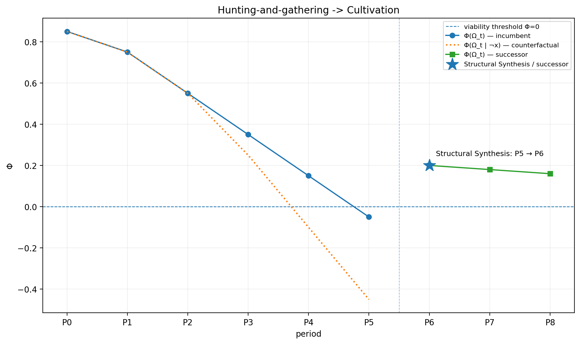
Structural Dialectics modeled viability path for hunting-and-gathering to cultivation, with synthesis on P5 to P6 — Figure 1. Hunting-and-gathering → cultivation: modeled incumbent viability, counterfactual dependence, and the P5 → P6 transition.

The synthesis marker appears at P6 because P5 is the originating period on which the transition condition Syn₅(x) evaluates, whereas P6 is the period in which the viable successor state Ω̂^x₆ is realized. The successor continues across the simulation window with Φ = 0.200 at P6, Φ = 0.180 at P7, and Φ = 0.160 at P8.

The sequence illustrates the distinction between admissibility, necessity, evidential support, realization, and successor viability. None of these conditions alone constitutes a completed synthesis.

5. Captive-Supply-Dependent Coercion → Alternative Labor Institution

The second example considers a transition from a captive-supply-dependent coercive labour arrangement toward an alternative labour institution. It is used as a historical analogy rather than as a quantitative reconstruction of a particular labour market.

The incumbent remains viable through P3 (Φ = 0.100) and crosses below the viability boundary at P4 (Φ = −0.050), where the candidate becomes admissible and counterfactual viability drops to −0.150 (dependence d₄ = 0.100). Because the incumbent is non-viable and an admissible alternative exists, P4 satisfies the diagnostic condition for Phase Inversion.

At P5 incumbent viability deteriorates further to −0.150, with counterfactual viability falling to −0.350 (dependence d₅ = 0.200). With admissibility maintained, the posterior probability reaches 0.607 against a threshold of 0.600, establishing warrant under Phase Inversion. The transition is scheduled across the P5 → P6 edge, producing a viable successor state with Φ = 0.150 at P6, Φ = 0.130 at P7, and Φ = 0.120 at P8.

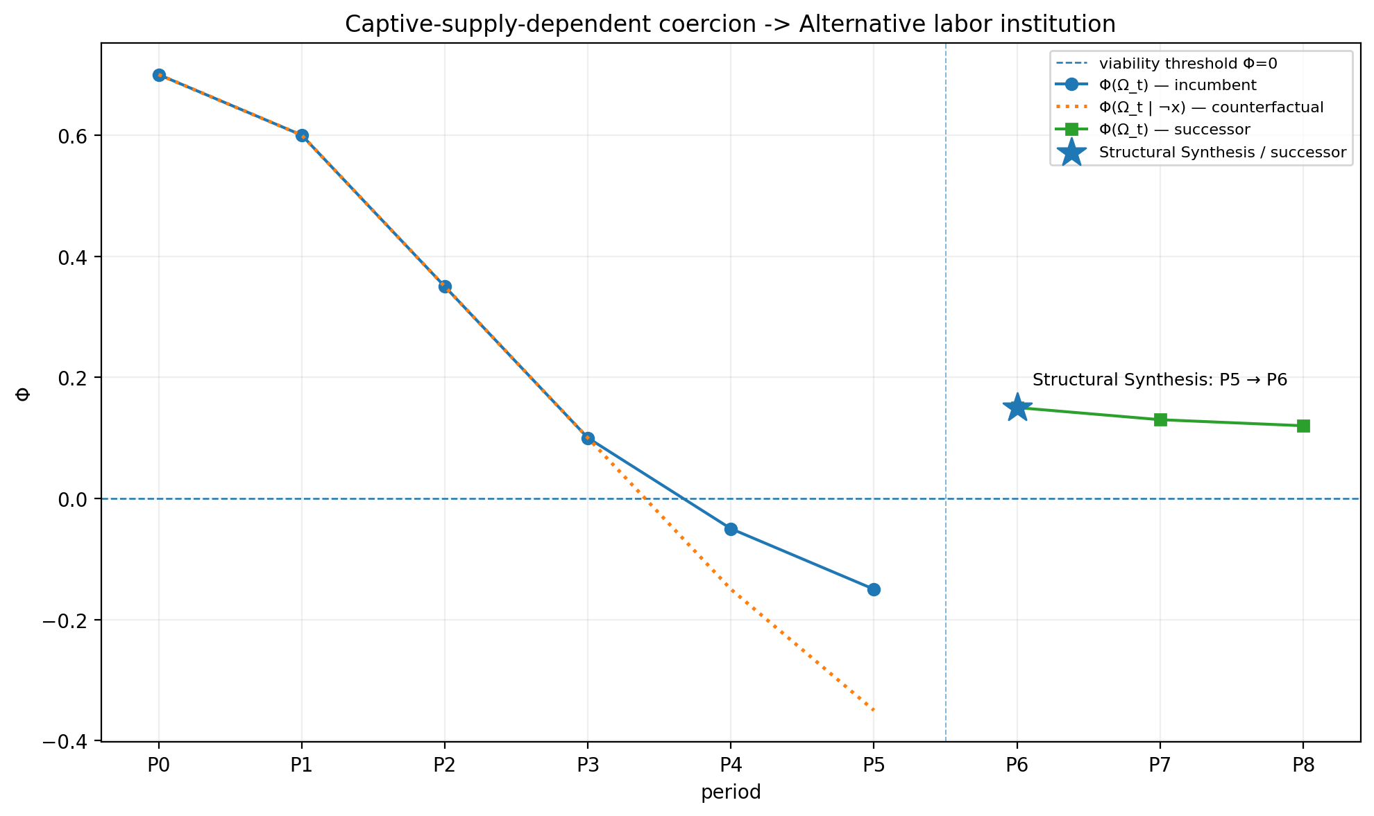
Structural Dialectics modeled viability path for captive-supply-dependent coercion to an alternative labor institution, with transition on P5 to P6 — Figure 2. Captive-supply-dependent coercion → alternative labour institution: modeled crisis, evidential support, transition, and successor viability.

The example shows why incumbent failure and institutional replacement are separate questions. The disappearance of viability does not by itself establish an admissible alternative, and admissibility does not by itself establish warrant or realization.

6. Serfdom (Domar Constraint) → Capitalist Tenancy

The third example considers serfdom under a Domar-style constraint and a transition toward capitalist tenancy. As with the preceding examples, the numerical parameters illustrate the formal mechanism rather than reconstructing the historical transition quantitatively.

The candidate becomes admissible at P5. At P5 the incumbent remains viable with Φ = 0.050, but removing the candidate drops counterfactual viability to −0.150 (dependence d₅ = 0.200). Because the candidate is necessary for incumbent viability, P5 produces the diagnostic condition Instability. At P6 the incumbent viability falls to −0.150 with a counterfactual value of −0.500 (dependence d₆ = 0.350), entering Phase Inversion. The posterior probability reaches 0.827 against a warrant threshold of 0.600, establishing warrant.

The transition occurs on the P6 → P7 edge and produces a viable successor state with Φ = 0.250 at P7, continuing to Φ = 0.230 at P8.

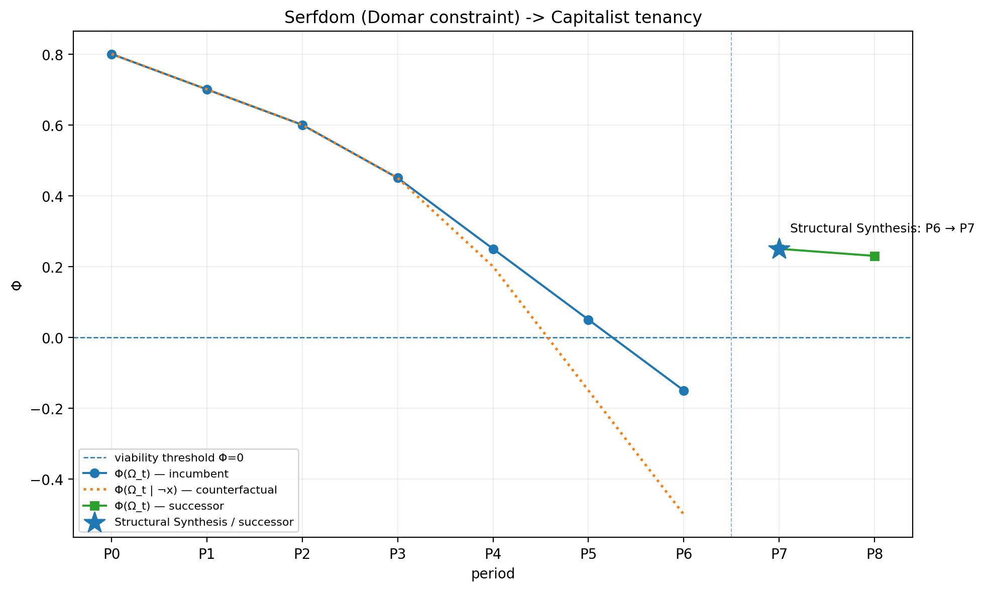
Structural Dialectics modeled viability path for serfdom under a Domar constraint to capitalist tenancy, with transition on P6 to P7 — Figure 3. Serfdom (Domar constraint) → capitalist tenancy: the modeled P6 → P7 transition and viable successor.

The case separates evidential support from transition. A high posterior does not itself produce the successor. The successor appears only when the transition rule generates it.

7. Capitalism and Demography: Incumbent Viability

The capitalism-and-demography example does not specify a candidate transformation. It therefore evaluates incumbent viability only. The predicates of possibility, necessity, warrant, realization, and synthesis are not applied to a particular alternative.

The normalized viability function is:

Φ_capitalism = 0.5n + g − δ − Δ(K/L) + 0.15

n: modeled demographic-growth term
g: productivity-growth term
δ: fixed normalized demographic-pressure parameter, set to 0.010
Δ(K/L): change in capital-labor ratio (capital deepening) used by the simulation
0.15: fixed normalized baseline contribution

In the simulation, demographic growth declines steadily from n = 0.030 at P0 to 0.000 at P6–P8, while capital deepening increases from Δ(K/L) = 0.020 at P0 to 0.310 at P8 (with δ fixed at 0.010). Figure 4 compares the resulting viability trajectories under sustained productivity growth (g = 0.20, where viability remains positive through P8 at Φ = 0.030) versus zero productivity growth (g = 0, where viability crosses into non-viability at P5 with Φ = −0.048, falling to −0.170 at P8).

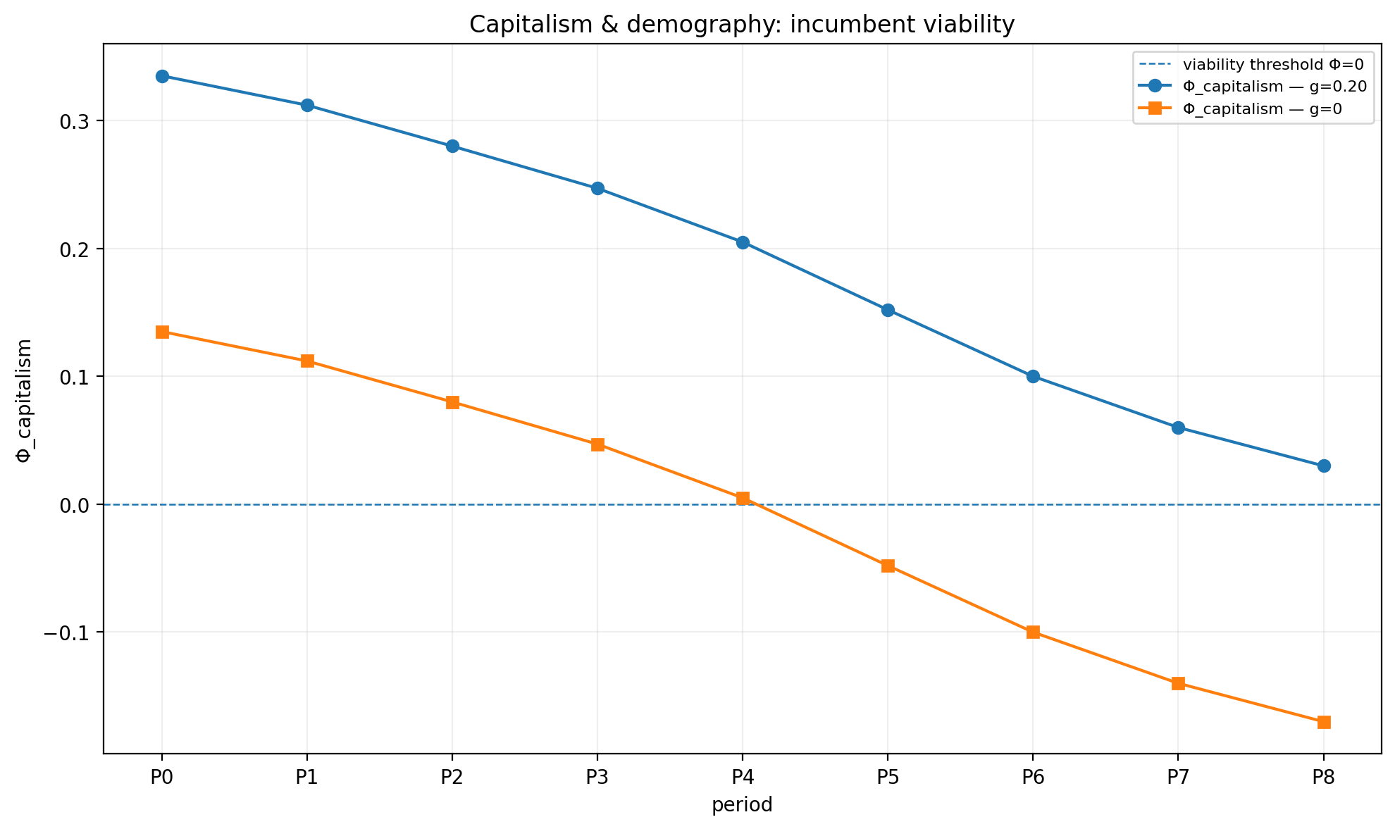
Structural Dialectics capitalism and demography incumbent viability comparison — Figure 4. Capitalism and demography: incumbent viability under two productivity-growth assumptions across P0–P8.

The figure is a parameterized comparison of viability. It is not a forecast of the future trajectory of capitalism.

8. Verification and Scope

The numerical implementation checks the internal relations specified by the model. For each transition scenario it checks:

that the counterfactual equals Φ(Ω_t) − d_t(x);
that possibility and the incumbent-viability condition are satisfied when necessity is reported;
that the posterior is calculated from the stated prior and likelihood values;
that warrant is reported only when the posterior threshold is met alongside either necessity or Phase Inversion;
that the scalar transition rule produces the specified successor viability when the transition is enabled;
that synthesis requires warrant, realization, and successor viability;
that the successor becomes the current state after a successful transition;
that incumbent-specific diagnostics are not carried over to the successor state.

The verification concerns the arithmetic and logical consistency of the specified model. It does not demonstrate that the model’s assumptions, parameters, or historical analogies are empirically correct.

The historical examples therefore remain open to empirical and historiographical evaluation. In particular, the numerical values do not establish historical dates, causal magnitudes, or empirical probabilities.

9. The Temporal Structure of Synthesis

The distinction between an event and the state produced by that event is central to the framework. If synthesis occurs at t, then:

Syn_t(x) → Ω_t+1 = Ω̂^x_t+1

The event belongs to the transition edge t → t+1. The successor belongs to period t+1. Thus a chart may place a synthesis marker at P6 while identifying the transition as P5 → P6.

After the transition:

Ω_t+1 := Ω̂^x_t+1

The successor is then treated as the new incumbent state. Counterfactuals concerning the former incumbent do not automatically carry over to the successor.

This distinction prevents two errors. The first is to treat synthesis as though it were a state that persists across periods. The second is to treat the successor as another observation of the institutional arrangement that preceded it.

10. The Central Distinction

Possible ≠ Necessary ≠ Warranted ≠ Realized ≠ Synthesized.

Possible: the candidate is structurally admissible.
Necessary: the candidate is admissible, the incumbent is viable, and removing the candidate makes the incumbent non-viable under the specified counterfactual.
Warranted: the candidate is necessary or admissible under Phase Inversion, and its posterior probability meets the specified evidential threshold.
Realized: the actual successor satisfies Ω_t+1 = F_Ω(Ω_t, E_t, U_t, x), so the full structural state generated by the transition is realized.
Synthesized: the candidate is warranted, the transition is realized, and the resulting successor is viable.

These distinctions separate structural admissibility from structural dependence, evidential support from occurrence, and occurrence from successful institutional replacement. A contradiction or crisis does not determine its resolution. Evidence does not itself produce a transition. A realized transition does not guarantee that the resulting state will remain viable.

11. Conclusion

Structural Dialectics treats institutional transformation as a sequence of formally distinguishable claims. Possibility concerns admissibility. Necessity concerns the dependence of an incumbent on a candidate under a specified counterfactual. Bayesian warrant adds an evidential condition. Realization concerns the transition from one state to another. Synthesis requires the resulting state to be viable.

The distinction between these conditions matters because historical transformation is not exhausted by the presence of contradiction or crisis. An institutional arrangement may become unsustainable without a viable alternative being available. An alternative may be available without being necessary. A necessary alternative may lack sufficient evidential support. A well-supported alternative may fail to be realized. And a realized transition may produce a successor that is itself unstable.

The temporal structure follows directly from this logic. Synthesis is an event on the transition from t to t+1; the successor becomes the current state at t+1. The numerical examples illustrate this structure using normalized values rather than quantitative reconstructions of historical processes.

The claim is that institutional transformation should not be described as a single condition when the relevant questions concern admissibility, dependence, evidence, occurrence, and viability. Keeping those questions distinct makes it possible to say exactly what a formal model establishes and what it leaves open.

All numerical examples in this post use normalized simulation values. They are illustrative model outputs rather than historical measurements.